Flight Planning and GSD Calculator (Beta)

Posted in Setup Operation, Setup Operations, Setup Operations, Setup Operations | Tagged Canon 5D Mark II, Photogrammetry, Photoscan, Photoscan Pro

Nikon D200 IR Calibration Values

Nikon D200 IR Calibration

Below are camera calibration values for the CAST Nikon D200 IR camera with Nikkor 28 mm lens. For projects requiring highest accuracy it is recommended that you perform your own calibration, otherwise these values can be used.

PhotoModeler v2012 Calibration Values (August 2013, F-stop of f/8, overall RMS 0.218 pixels):
– Focal Length: 29.630373 mm
– Xp: 11.836279 mm
– Yp: 8.051145 mm
– Fw: 23.999451 mm
– Fh: 16.066116 mm
– K1: 1.435e-004
– K2: -1.481e-007
– P1: 5.659e-006
– P2: -1.311e-005

Calibration Values for PhotoScan (converted from PhotoModeler values using Agisoft Lens):
– fx: 4.7804273068544844e+003
– fy: 4.7803319847309840e+003
– cx: 1.9096258642704192e+003
– cy: 1.2989255852147951e+003
– skew: -8.0217439143733470e-004
– k1: -1.2545715047710407e-001
– k2: 1.5266014429827224e-001
– k3: -7.6547741407995973e-002
– p1: 3.5948192692070413e-004
– p2: -1.5418228415832919e-004

Posted in Uncategorized | Tagged Camera Calibration, Nikon, Nikon D200 IR

Pseudo-NDVI from Nikon D200 IR Images

Nikon D200 IR Light Transmission

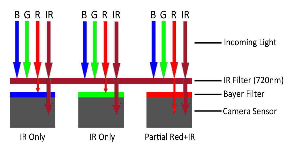
Because of the light transmission properties of the filter installed in the CAST Nikon D200 IR DSLR camera, it is possible to isolate infrared and red light into separate channels. These channels can then be used to generate an NDVI image using the well known formula:

NDVI = (NIR – Red) / (NIR + Red)

We’re calling this pseudo-NDVI for a couple reasons; 1) the IR filter installed only captures a portion of the visible red (probably less than half), so this bit of information is relatively weak, and 2) our method of isolating the “reflected red” (Band1 – Band3) is overly simplistic. However, we have tried more complicated methods (e.g. principal components, also averaging bands 2 and 3) but results did not improve. Without more work, the results of this process should not be compared to calibrated NDVI images.

1. Load (individually) bands 1 and 3. Band 1 represents Red+IR, Band 3 is IR only.

Nikon D200 IR Bands 1 and 3

2. Run the Raster Calculator tool to produce a “reflected red” raster using the following raster math:
Band1 – Band3

Nikon D200IR “Reflected Red”

3. Run the Raster Calculator tool to produce NDVI raster using:
(Float(“Band3”) – Float(“ReflectedRed”)) / (Float(“Band3”) + Float(“Reflected Red”))

Nikon D200IR Quasi NDVI

Note: If you don’t use the Float functions in step 3 you end up with integers (-1,0,1), which are useless.

Posted in Setup Operations | Tagged NDVI, Nikon D200, Nikon D200 IR

Specific Settings for Nikon D200 and Close-Range Photogrammetry

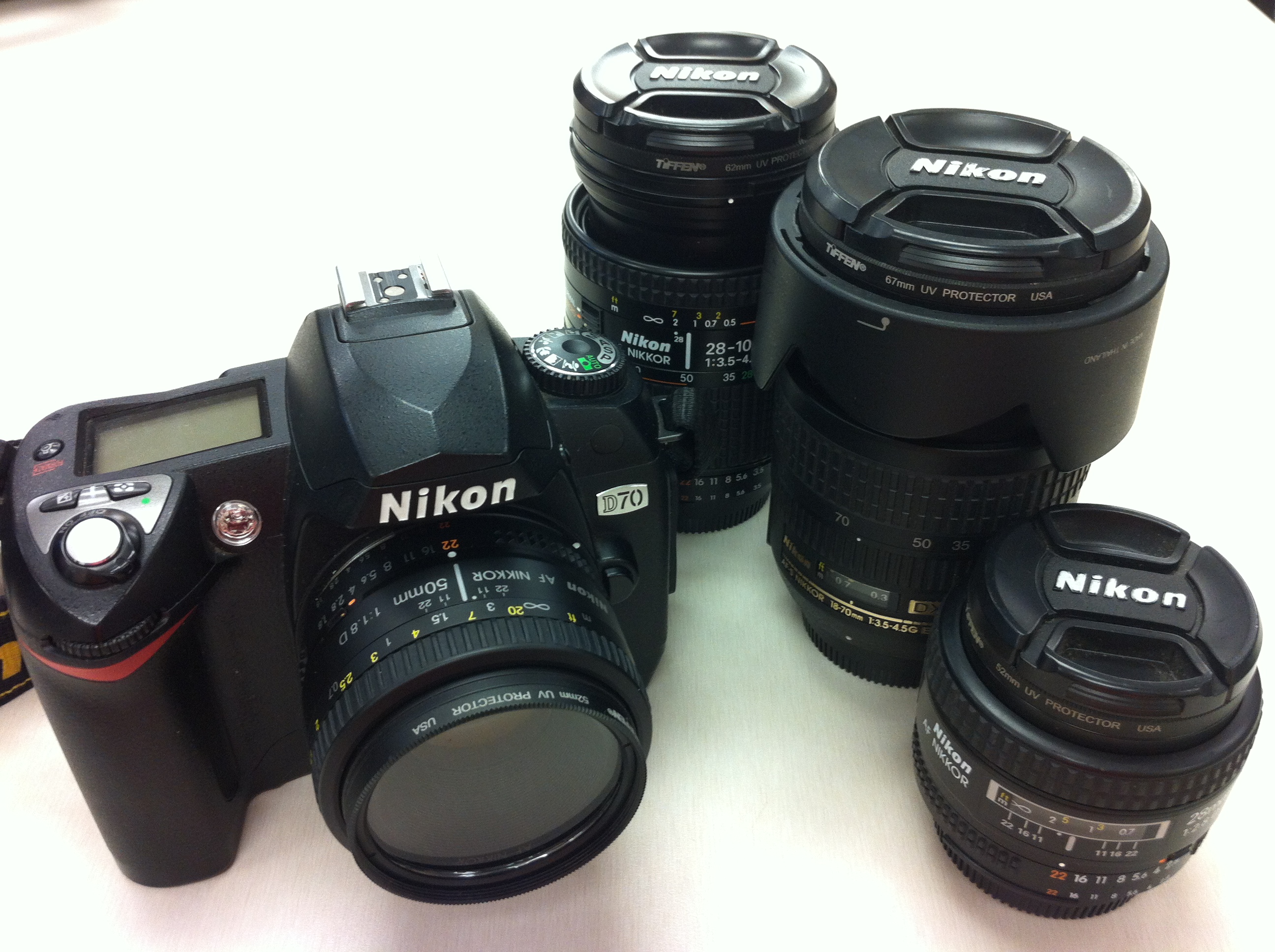
Nikon D70 and Nikkor lenses

Along with the generic advise given in the Acquire Images for Close-Range Photogrammetry and Custom White Balance for Nikon D200 IR posts, here are some important settings to consider when using the standard or IR modified Nikon D200 cameras:

– Rotate Tall: Set “Rotate Tall” to Off if the images are to be used for photogrammetry or GIS applications

– Image Quality: Use either the “NEF (RAW)” or “NEF (RAW)+JPEG” image quality setting. Capturing RAW images will preserve all image information and give you much more control over editing later

– Image Size: Set to “Large 3872×2592/10.0M”

– Optimize Image: Use these “Custom” settings and adjust as needed:

–Image Sharpening = None
–Tone Compensation = Normal (0)
–Color Mode = III
–Saturation = Normal (0)
–Hue Adjustment = 0
–Make sure you select “Done” after making adjustments to theses settings or they will be lost.

– Color Space: Should be set to “sRGB”

– JPEG Compression: For highest quality set to “Optimal Quality”

– RAW Compression: If memory card space is not an issue, set to “NEF (RAW)” for no compression. Otherwise turning on compression will cut the size of RAW images from 16MB to 9MB

– Intvl Timer Shooting: This setting can be used to take a predetermined number of images with a certain amount of time between each shot. To use this setting, three setting must be set:

1. Start: Two options exist including “Now” (starts taking images right away) or “Start Time” (allows you to set a time (e.g. 13:00, aka 1pm). If using Start Time, make sure the cameras time setting is correct
2. Interval: Sets the amount of time between each interval using hours, minutes, and/or seconds (one second minimum)
3. Select Intvl*Shots: This setting ask you to set 1. the total number of intervals and 2. number of images at each interval. If mounting the camera to the octocopter for example, one could set the Interval to 10 seconds, the total number of intervals to 50, and the number of images at each interval to two. This would result in 100 total images, with two at each of the 50 positions (interval)

Posted in Setup Operations, Setup Operations | Tagged close range scanning, Nikon, Nikon D200, Photogrammetry

Custom White Balance for Nikon D200 IR

Nikon D200IR Custom White Balance Results

Because some red light is transmitted by the IR filter, any of the standard white balance settings will produce reddish images. A custom white balance using the “White Balance Preset” option can be used for better images. It’s important to note that the white balance setting is only applied to JPEG images saved on the memory card – RAW images are saved to the memory card exactly as they are recorded by the image sensor, without any processing. However, even when capturing RAW images, the image preview on the camera’s LCD will use the white balance setting, and will therefore be easier to evaluate exposure in the field.

To use the White Balance Preset option, follow these instructions to capture an appropriate custom WB image:

1. Hold down the “WB” button and rotate the rear wheel to select the “PRE” setting, release WB
2. Hold down the “WB” button until “PRE” begins to flash
3. Use the shutter release button to capture a photograph of healthy green grass in similar lighting as your intended subject (e.g. direct sun)
4. The camera should indicate “Good” or “No Gd” – if “No Gd” try again
5. If the camera indicates Good, take a test image to visually check your white balance

Posted in Nikon D200 IR, Setup Operations

Cleaning Scans in Polyworks IMAlign

Coming Soon!

This document is under development…Please check back soon!

Posted in Uncategorized

Basic Cleaning and Exporting in OptoCat

Coming Soon!

This document is under development…Please check back soon!

Posted in Uncategorized

Konica-Minota Vivid 9i – Check List

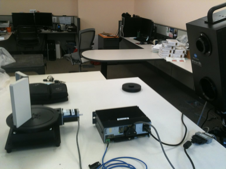
Note: The Konica Minolta VIVID 9i is best suited for indoor use. It will not work in direct or indirect sunlight. Any planned outdoor scanning should be done at night or under a blackout tent. The Minolta is also meant to be plugged in, so a generator or alternate power source is required when working outdoors.

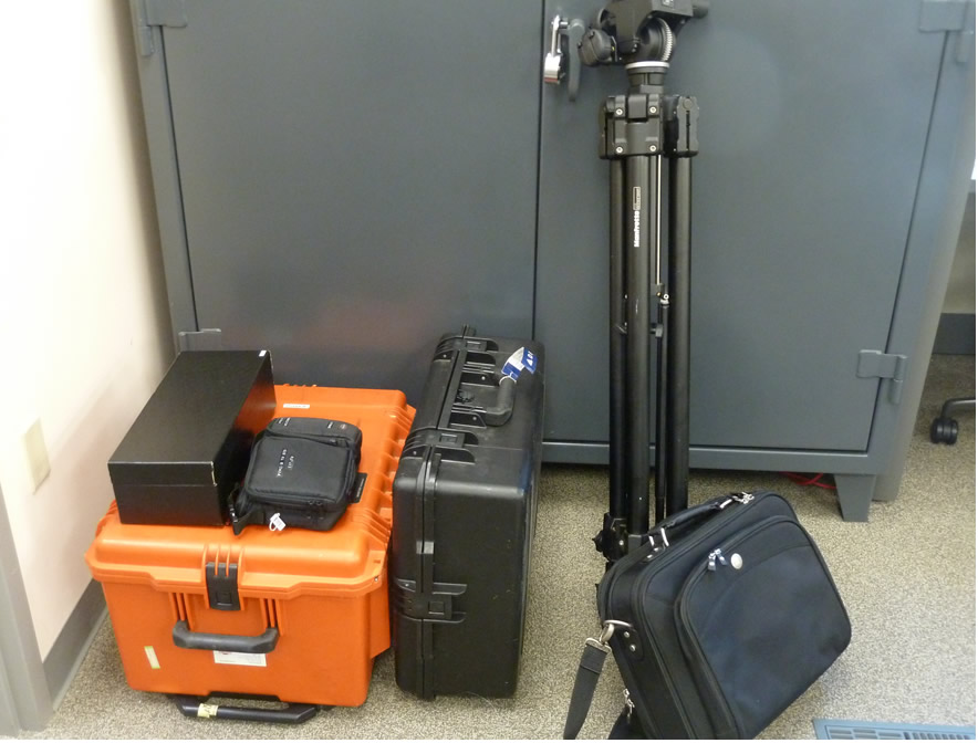
___ VIVID 9i Scanner (Large orange hard case)

___ Turntable – optional (Medium black hard case)

___ Manfrotto tripod

___ Laptop with Polyworks installed (with REQUIRED Plugins Add-on). If you are going to be off the network, then you must borrow a license from the Polyworks license server to be able to use the software. Note: The laptop must be 32 bit with Windows XP with a PCMCIA card slot and serial connection. The Panasonic Toughbook is most commonly used with VIVID 9i and has the required configuration.

___ Black lens box

___ Small black case with cables and accessories

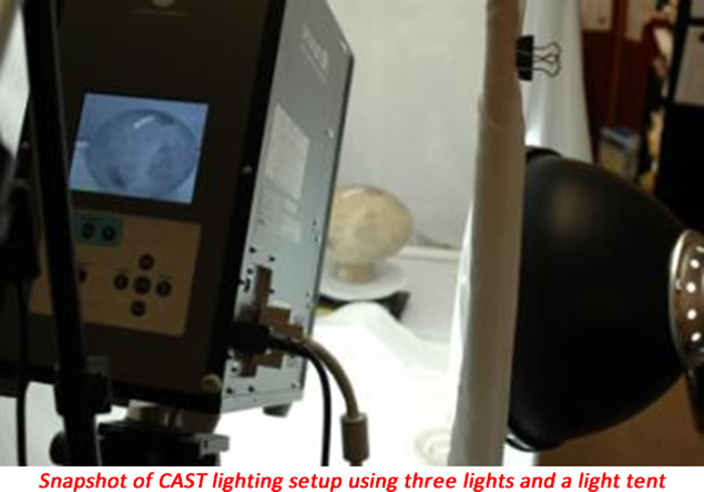
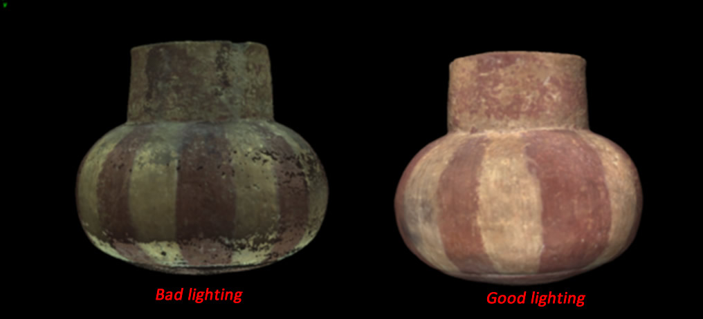
___ Additional lighting – optional (not shown above) Note: In addition to capturing surface information and detail of an object, the VIVID 9i also captures color (RGD) data. If the color properties of an object are important to your project, then we advise to use additional lighting to ensure more accurate color capture. CAST has a three light setup that uses white flicker-free flourescents that is available for checkout. If color is important – use good lighting (it can make all the difference).

Posted in Uncategorized

Konica-Minota Vivid 9i – Scanner Settings & Data Collection

This document guides you through scanner settings and collection procedures using the Konica-Minolta Vivid 9i, a turntable and Polyworks IMAlign software.
Hint: You can click on any image to see a larger version.

[wptabs style=”wpui-alma” mode=”vertical”] [wptabtitle] CALIBRATION [/wptabtitle]

[wptabcontent]

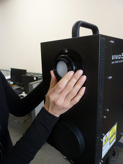
1. White Balance Calibration: Before you begin scanning, you need to perform the white balance calibration on the scanner. Make sure the lighting conditions in your environment are set to what they will be during the scanning process.

A. Next, remove the white balance lens from the lens box and screw it onto the top front of the scanner.

B. Press the Menu button the back of the scanner and select White Balance and press Enter. Under the White Balance menu, choose Calibration and press Enter. Do not touch or pass in front of the scanner while it is performing the calibration.

C. When the calibration is complete, remove the white balance lens and put it back in the lens box. You are now ready to begin your scanning project.

[/wptabcontent]

[wptabtitle] TITLE OF SLIDE [/wptabtitle] [wptabcontent]
2. Open Polyworks IMAlign (v 10.1 in this example) and select the Plugins menu – Minolta – VIVID 9i – Step Scan. The One Scan option is used if you are not using the turntable. If you do not see the Plugins menu, you will need to install the Plugins Add On from the Polyworks installation directory.

3. When the VIVID 9i window opens, you should see a live view from the scanner camera. Select the Options button on the right. Under Scan Parameters, select Standard Mode. Extended mode offers a greater scan range however it limits noise filtering operations. Standard mode should work for most projects. The number of scans are the number of passes the scanner makes per scan position. From the manual: “It averages the data from each pass to produce a single scan file therefore more scans theoretically will give you the most accurate data. We recommend 3 or 4 scans, however if time constraints are an issue then this number may be lowered.

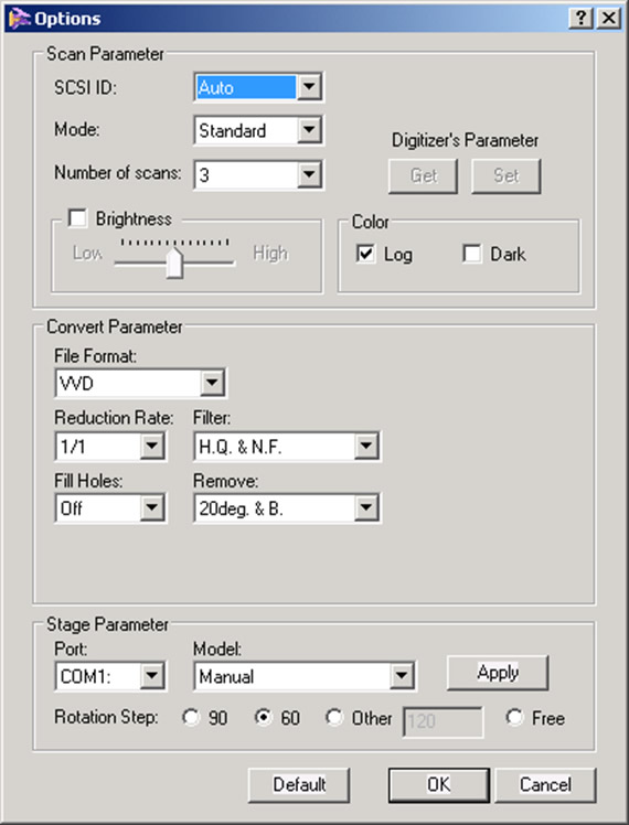
4. Under Convert Parameter, check the VVD File Format and a Reduction Rate of 1/1 (No data reduction). Under filter, select H.Q. & N.F. (High quality and noise filter). This is the highest filter setting and is most effective for minimizing scanner noise. Also, make sure Fill Holes is Off and under Remove, it is generally advised to select 20deg & B. (20 degrees and Boundary). This last parameter removes data around the perimeter of a scan that tends to be less reliable. In previous experiences, it was noted the data around the scan edge often curves up creating an artificial lip in the data. Researchers found that increasing the Remove parameter to the highest setting, removed the “scan edge lip.” All of the settings above are just suggestions and may need to be altered to suit individual project needs.

5. Under Stage Parameter – Model, select Parker 6105 (Fast); this selects the correct turn table model. Finally select the desired Rotation Step. A Rotation step of 60 is suggested which will result in collecting 6 scans per object rotation.

6. Hit Apply and then OK.

7. Back in the VIVID 9i Window, select the Stage Apply button to apply the stage parameters. Next, we will calibrate the turntable by using the black and white calibration charts found in the turntable case.

8. The smaller chart is used with the tele lense and the larger chart is used with both the mid and wide angle lenses. Place the appropriate calibration chart on the system turntable facing the scanner. The smaller chart has two pegs that fit associated holes on the turntable. The larger chart also has two smaller pegs that rest in a recessed ring on the turntable. In either case, it is important for the center of the chart to rest in the center of the turntable and for each chart to be completely upright. The black line that runs down the center of each chart is used to identify the center axis of the turntable which is then used to coarsely align or register the scans from a single scan rotation. In this example, the tele lense and small chart will be used.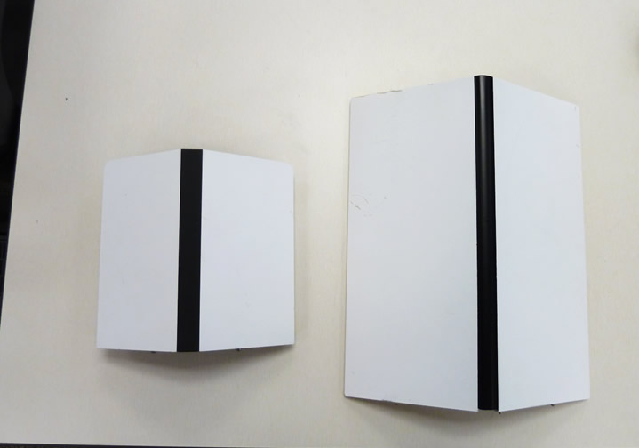

9. You should now see the scanner chart in the live view window. It is recommended to fill the view with the scan chart as best as possible. You may need to adjust the scanner position and rotation to achieve the correct view. NOTE: You will not be able to move the scanner after you perform the turntable calibration. If you do move the scanner after this step, then the turntable will need to be re-calibrated.

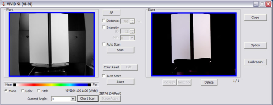
10. Next, hit the Chart Scan button. The scanner will then scan the chart and indicate whether or not the calibration was successful. It is not necessary to store the chart scan.

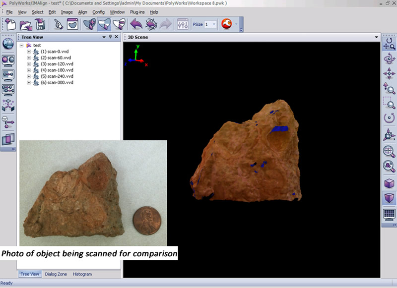
11. You are now ready to begin scanning. Place the desired object on the center of the turntable. It is advised to perform a single scan to test system perameters before completing a scan rotation. First, select the AF (Auto Focus button). This auto focuses the scanner camera and determines the object’s distance from the scanner, displaying the value in the Distance box. The Distance value can be altered to acquire object data at a specified distance. Next, press the Scan button. Once completed the scan should appear in the Store window on the right. Check the scan for any anomalies such as holes, poor color, etc. If you wish to keep the scan, you MUST click the Store button. If you do not click the Store button, the scan will be overwritten. If you are happy with the scan results, then you are ready to proceed with a scan rotation.

12. To perform a scan rotation, first select the Auto Scan and Auto Store options. Next, press the Scan button. The scanner will perform 6 scans rotating 60 degrees between each scan and will automatically store the results in the IMAlign project. Once the scans are complete, click in the IMAlign project window to view the results.

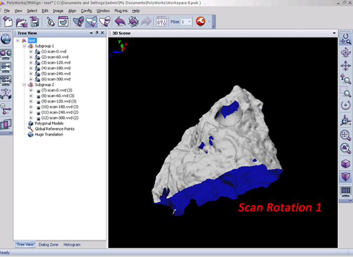
13. The six scans are displayed in the Tree view (table of contents) on the left with the name “scan” followed by a suffix indicating the scan angle (0, 60, 120, etc…) and represent one complete scan rotation. These scans have been roughly aligned to one another based on the central axis of the system’s turntable. We recommend to clean and align scans as you go as it takes little additional time and it ensures that all of the required data has been captured (and all holes/voids have been filled in).

14. Using the middle mouse button, select and delete any data that are not associated with your scan object. Next, make sure all of your scans are unlocked and run a Best Fit alignment. The Best Fit operation is an iterative alignment that produces a more accurate alignment between the scans.

15. Now that the scan rotation has been cleaned and better aligned, prepare for the next scan rotation by first locking all of the scans of the first rotation (select all in the Tree View, right click and select Edit – Lock or use Ctrl+Shft+L) and then by grouping the scans together (select all in the Tree View, right click and select Group). Now observe the data that you have collected, note holes or voids in the digital object, and identify what areas need to be scanned next. If you are scanning a large object, perhaps you will need to perform another scan rotation to acquire more of the object or if it’s a smaller object, perhaps a few single scans are needed in order capture the bottom and top views of the object. Reposition the object on the turntable to prep for the next scan sequence.

16. Next, return to the scan window and complete another scan/scan rotation. In this example, we will complete another scan rotation in order to show how align two rotations to one another.

17. Because the object has been repositioned, it is always good to Auto Focus (press the AF button) before each scan/scan rotation. Complete the second scan or scan rotation.

18. In the IMAlign window, you may have to hide the first scan rotation (simply middle click on the group name or right click the name and select View – Hide or use Strl+Shft+D) to more easily view the new data. Go ahead and delete any extraneous data from the scene and group the scans from the second rotation (select all, right click and select Group).

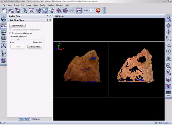
19. To align the second rotation to the first rotation, first unhide the first rotation (middle click the group name or right click and select View – Restore or use Ctrl+Shft+R). Next select the split view alignment button and independly rotate each view so that they are roughly the same perspective of the scan object .

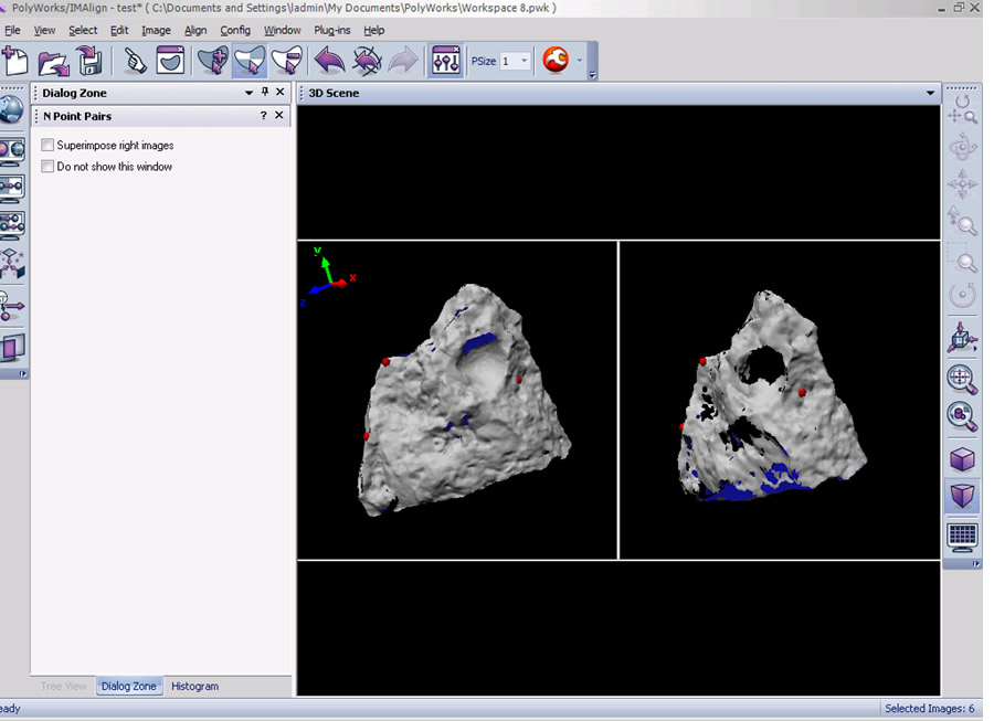
20. Now select the N Point Pairs button (Align Menu – N Point Pairs) and identify at least three pick points between the two views. Right click when complete and you should now see the second rotation roughly aligned to the first. Run a best fit alignment to optimize the alignment and then lock the second scan group. This is a very basic description of alignment in IMAlign, for more detail please refer to the Registering (aligning) Scan in Polyworks IMAlign workflow.

21.

Complete as many scans/scan rotations that are necessary in order to get a complete digital model of your object. Small holes can be holefilled with additional post processing in IMEdit.

22. Refer to the Registering (aligning) Scan in Polyworks IMAlign workflow for further details on scan alignment and the Creating a Polygonal Mesh using IMMerge workflow for more information on creating a polygonal mesh file in Polyworks.

[/wptabcontent]

[/wptabs]

Posted in Uncategorized

Konica-Minolta Vivid 9i – Setup with turntable

This document will guide you through setting up the Konica-Minolta for use with a turntable.
Hint: You can click on any image to see a larger version.

[wptabs style=”wpui-alma” mode=”vertical”] [wptabtitle] TRIPOD & MOUNT [/wptabtitle]

[wptabcontent]

1. Setup the scanner tripod. The tripod doesn’t have to be completely level but you want it to be stable so some degree of leveling is required.

2. Prep the scanner mount by pulling the black lever out, pushing up the gold pin, and then releasing the lever. This widens the slot where the scanner mount rests.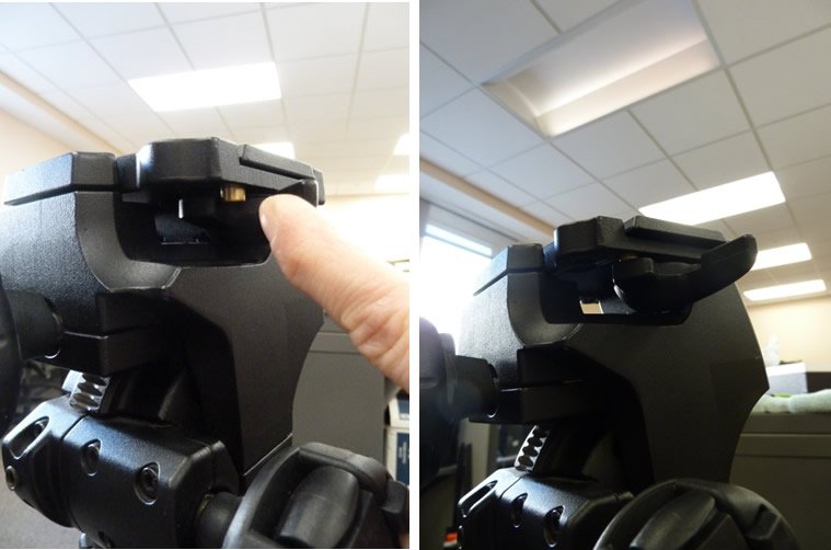

When done correctly, the lever will continue to stick out.

[/wptabcontent]

[wptabtitle] CONNECT SCANNER [/wptabtitle] [wptabcontent]

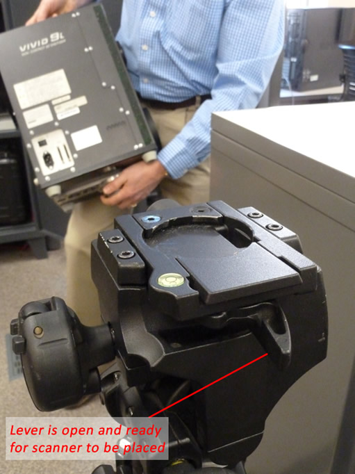
3. Place the scanner on the tripod until it locks into place (you will hear a ‘click’ sound when the mount has locked). Once the scanner has been mounted, ensure that your setup is stable.

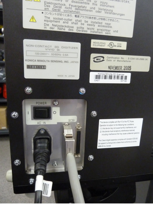
4. Remove the power cable and gray SCSI cable with the PCMCIA card adapter from the small black case. Plug the scanner power cable in and connect the SCSI cable. DO NOT TURN THE SCANNER ON.

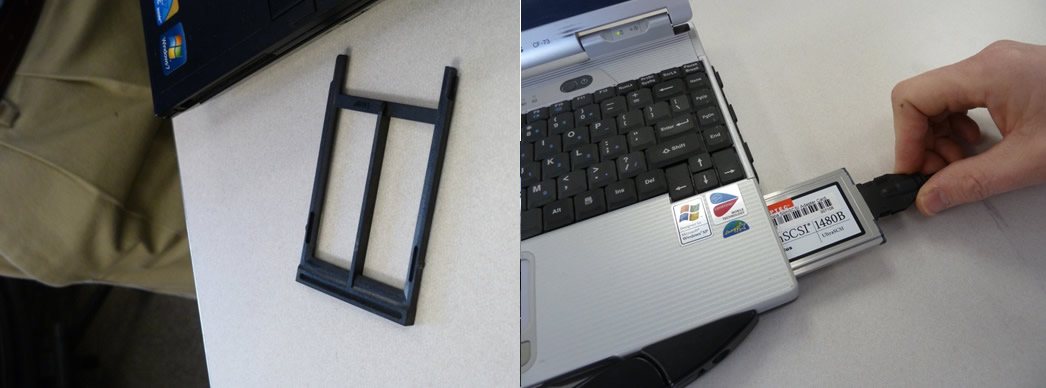
5. Remove the card insert from the PCMCIA slot on the laptop and plug the PCMCIA card into the laptop.

[/wptabcontent]

[wptabtitle] SETUP TURNTABLE [/wptabtitle] [wptabcontent]

6. Remove the turntable, black power box, and all cables from the black case. Set the two, black and white calibration charts to the side for now. Place the turntable approximately 1 meter (or slightly less) from the scanner with the corded end facing towards the front i.e. towards the scanner. The suggested scan range for the tele and mid lenses is .6 to 1 meter. When you begin scanning, the distance parameter will be displayed in the scan window. We generally suggest to keep the distance in the range of 700-800 mm to avoid data loss that can occur when an object is either too close or too far from the scanner.

7. Plug the gray cable from turntable into the black power box; also plug the power cable into the black power box. Next, take the blue serial cable and plug the green end (with 4 prongs) into the COM1 port on the black box. NOTE: Theprongs on the green end are directional and will face down.

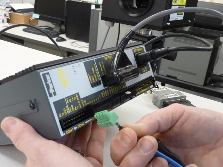
[/wptabcontent]

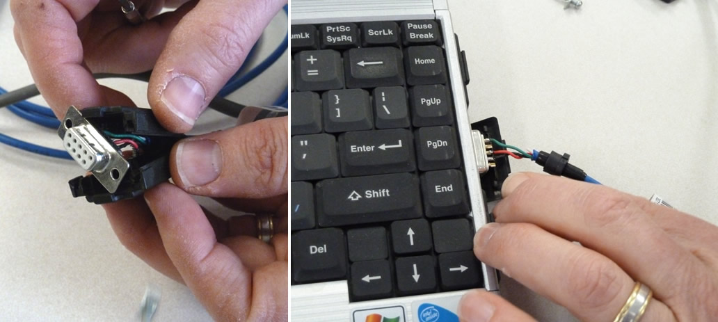
[wptabtitle] CONNECT LAPTOP [/wptabtitle] [wptabcontent]

8. Next, take the other end of the serial cable and plug it into the serial connection on the laptop. To work with a laptop, you will probably have to remove the black case around the plug end using a small screwdriver.

[/wptabcontent]

[wptabtitle] POWER UP SCANNER [/wptabtitle] [wptabcontent]

9. Once everything has been plugged in and you have the desired lens in place (see the Changing Lenses section in the final slides of this post if you need to change the scanner lens). Next power on the scanner. It will take a minute to load, when it is complete, it will display the following message on screen “Please open laser barrier and press any key.”

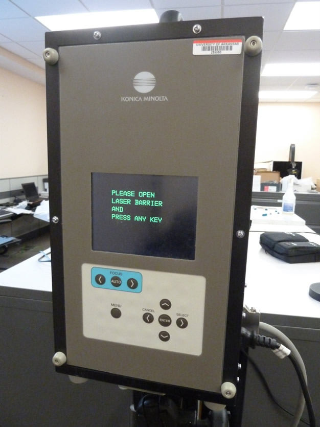
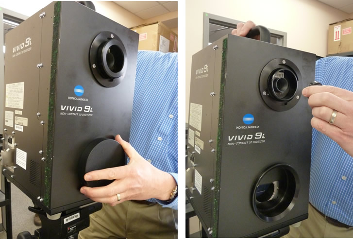
10. Next, pull the large round cap off of the front of the scanner (bottom) and remove the lens cap (top), and then press any button on the back of the scanner to continue.

[/wptabcontent]

[wptabtitle] OPEN POLYWORKS [/wptabtitle] [wptabcontent]

11. Next power on the laptop and log on. Note: It is important to power the scanner first and then the laptop so the connection is established.

12. Once everything has been turned on, open Polyworks on the laptop. Once the Polyworks Workspace Manager opens, open the IMAlign Module. Next, go to Scanners menu, and select Minolta – VIVID 9i. In the window that comes up, you should see a live camera view from the scanner (connection successful – hooray.) You are now ready to continue to the Konica-Minota Vivid 9i – Scan Settings post.

[/wptabcontent]

[wptabtitle] VIVID 9i LENSES [/wptabtitle] [wptabcontent]

Changing the Lenses on the VIVID 9i

The VIVID 9i comes with a set of three interchangeable lenses: tele, middle, and wide. The scanner’s camera array is fixed 640X480 pixels. Each lens offers a different field of view with the tele being the smallest. The FOV for each lens is provided below.

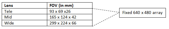
The tele lens offers the best resolution and is ideal for scanning objects smaller than a baseball or larger objects with a higher resolution. The mid lens works well for objects that are basketball size and was the lens predominantly used for scanning pottery vessels in the Virtual Hampson Museum project. CAST researchers generally do not recommend use of the wide angle lens.

[/wptabcontent]

[wptabtitle] CHANGING LENSES I [/wptabtitle] [wptabcontent]

A. To change the lens on the VIVID 9i, first make sure the scanner is turned off.

B. Next remove the lens that you wish to use from the lens box and its plastic bag.

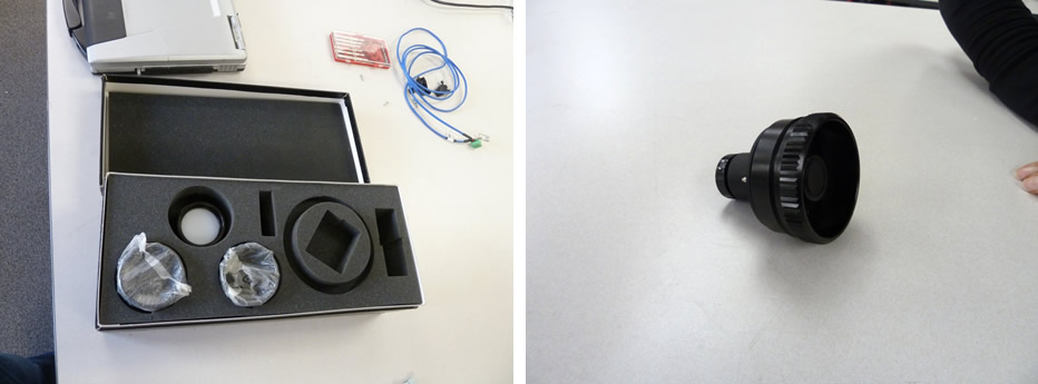
C. Next remove the lens protector and unscrew the lens that is currently on the scanner. IMMEDIATELY place the lens cap (located on the lens box) on the back of the lens.

NOTE: Every lens should always have 2 lens caps (one of the front and back of the lens) when the lens is not in use or is being stored.

[/wptabcontent]

[wptabtitle] CHANGING LENSES II [/wptabtitle] [wptabcontent]

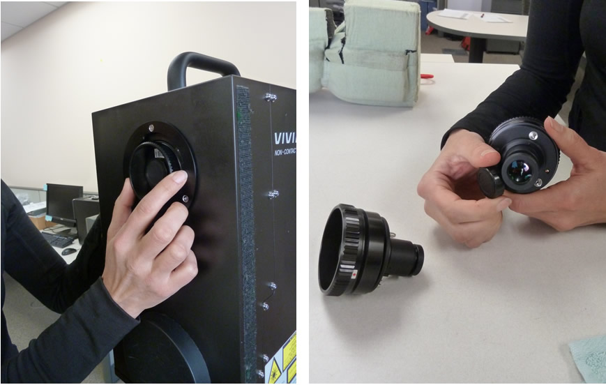
D. Remove the back lens cap from the desired lens and screw the new lens into the scanner by first lining up the red dots found on both the lens and the scanner.

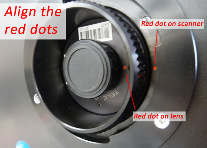
E. Replace the black lens protector on the scanner. Replace both lens caps on the newly removed lens, place in a plastic bag, and store in the lens box.

F. You are ready to begin scanning. Power on the scanner and continue with Step 9 on the ‘Power up Scanner’ Slide above.

[/wptabcontent]

[wptabtitle] CONTINUE TO… [/wptabtitle] [wptabcontent]

Continue to Konica-Minota Vivid 9i – Scan Settings.

[/wptabcontent]

[/wptabs]

Posted in Checklist | Tagged Archaeology/Historic Recordation, close range scanning, Data Collection, Konica Minolta, Polyworks, scanning range >5 meters

Leica GS15: Tripod Setup

This page will show you how to set up a tripod for use with a Leica GS15 GNSS receiver used as the base in an RTK survey or as the receiver in a static or rapid static survey.
Hint: You can click on any image to see a larger version.

[wptabs mode=”vertical”]

[wptabtitle] Hardware[/wptabtitle]

[wptabcontent]

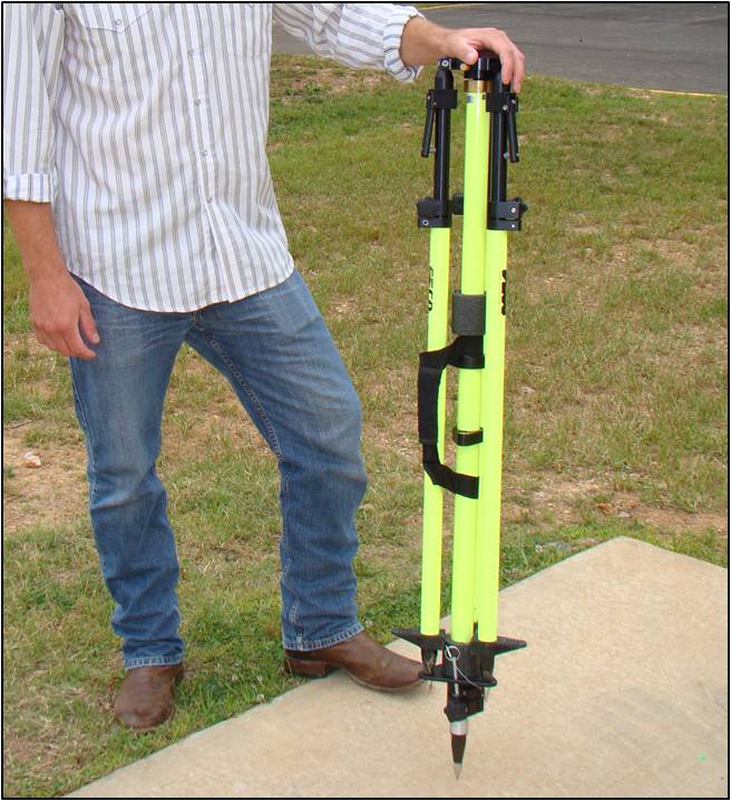
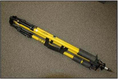
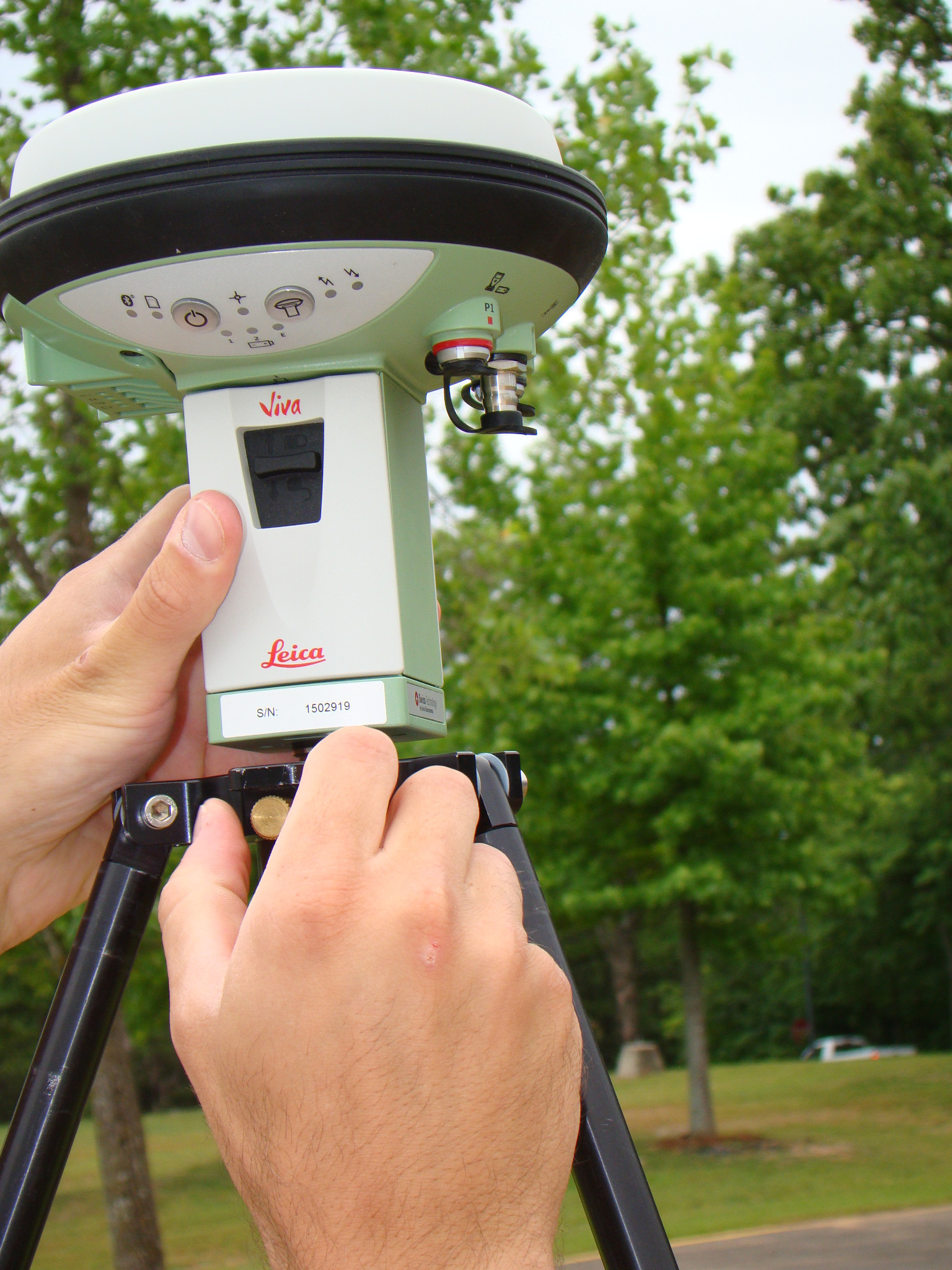
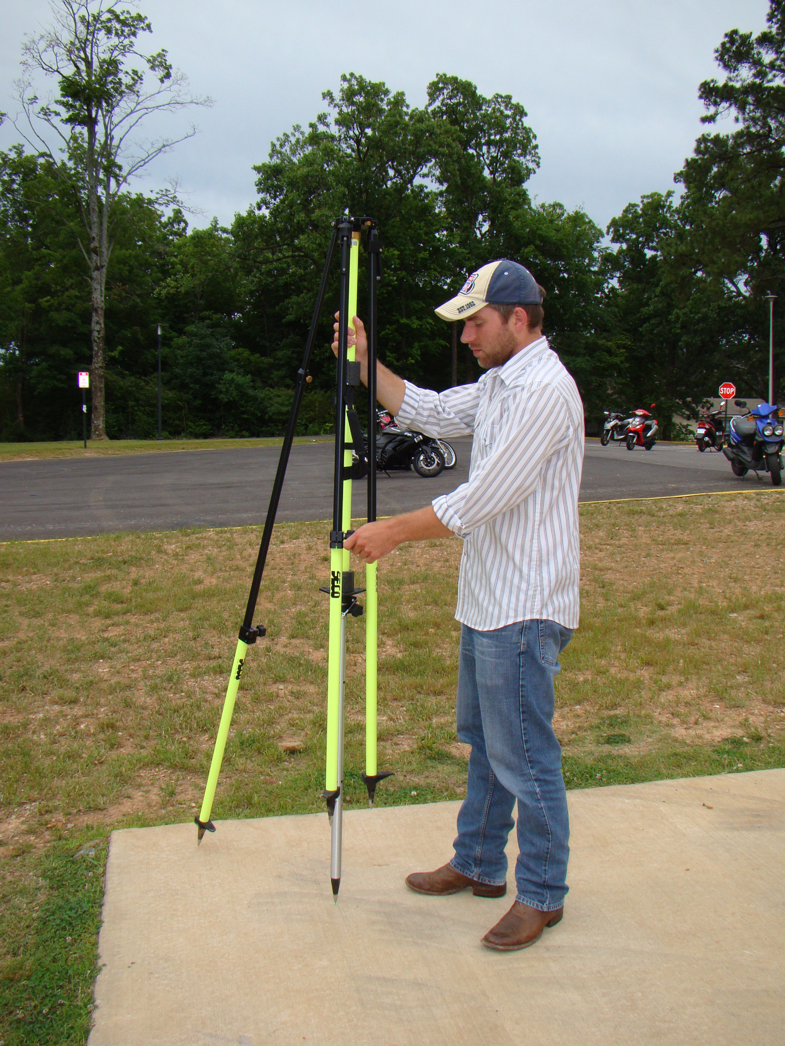
You will need a GS15 receiver, a brass tripod adapter, and one of the heavy duty, fixed height, yellow tripods.

[wptabtitle] Brass Adaptor[/wptabtitle]

[wptabcontent]

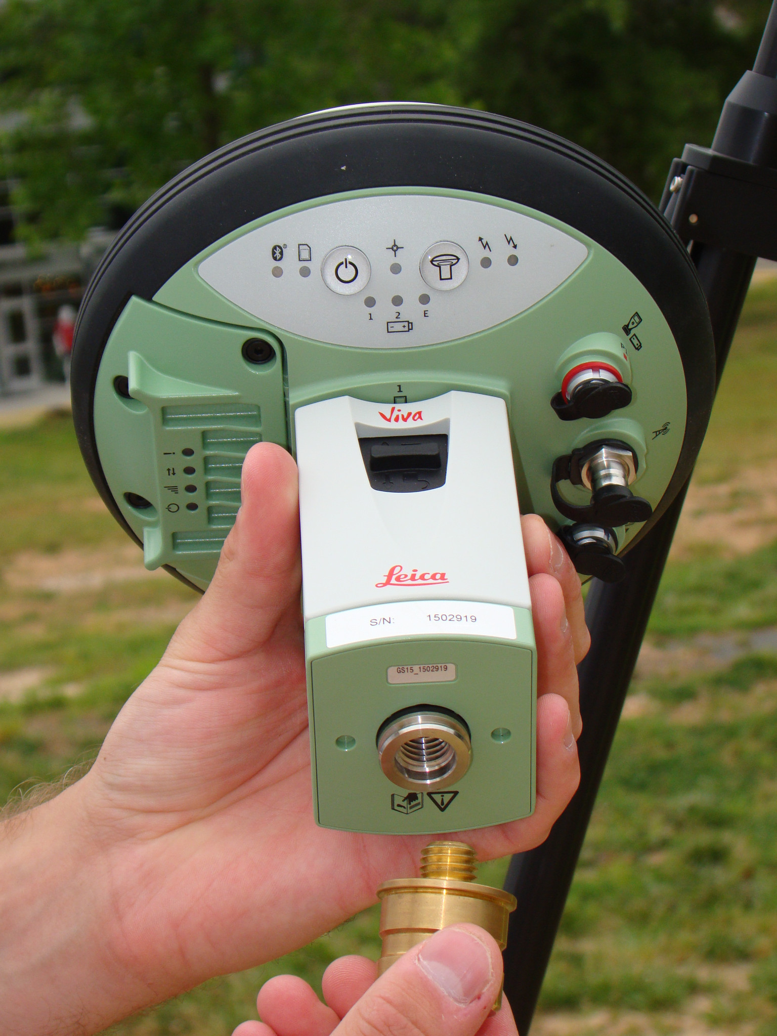
Screw the brass tripod adaptor into the base of the GS15.

Stand the fixed-height tripod on its center tip, loosen the brass thumbscrew in the side of the top mounting plate, insert the brass adapter on the antenna into the mounting hole, and then tighten the thumbscrew.

[wptabtitle] Extend Center Leg[/wptabtitle]

[wptabcontent]

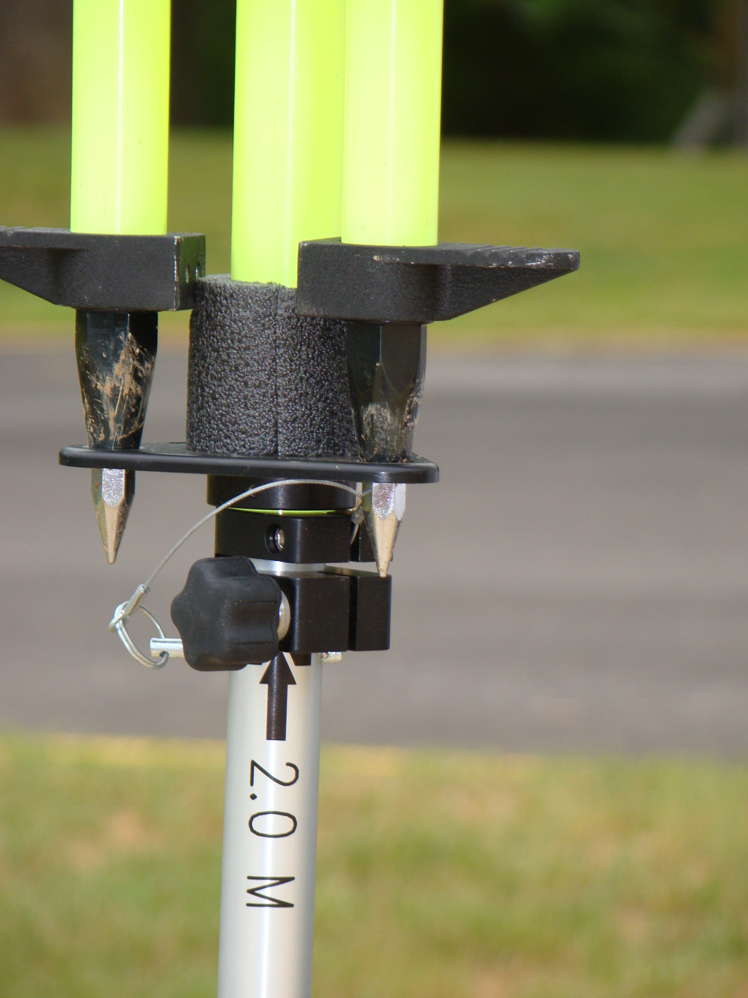
At the base of the tripod, flip the lever to release the center leg, and then extend it fully to the 2-meter mark.

There is metal pin attached by a wire to the base of the tripod – insert the pin through the holes in the rod at the 2-meter mark, then put the weight of the tripod on to the center pole so that the pin is pushed firmly against the clamp body. Now flip the lever to lock the clamp.

[wptabtitle] Position Tripod[/wptabtitle]

[wptabcontent]

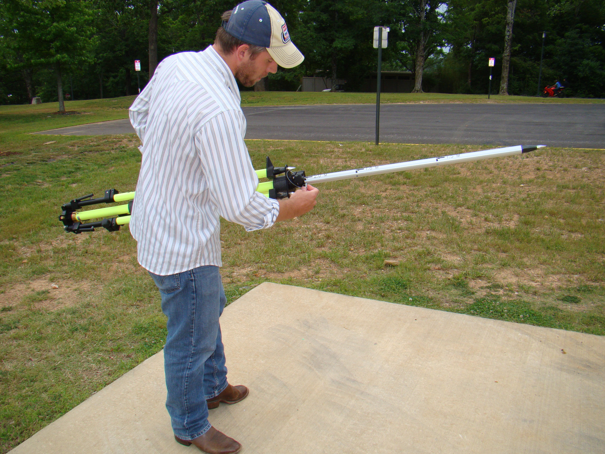
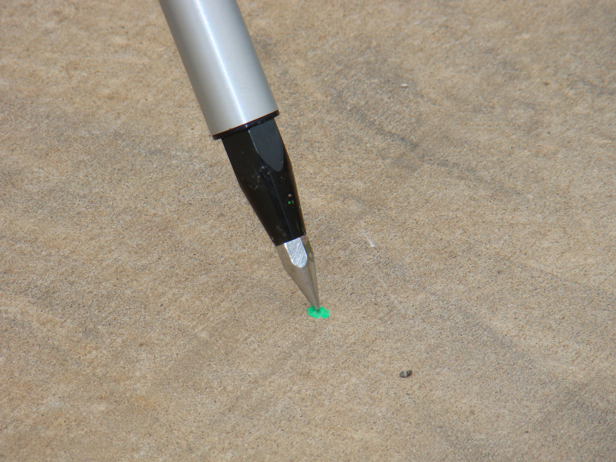
Carefully place the tip of the center pole at the exact spot on the ground that you wish to survey.

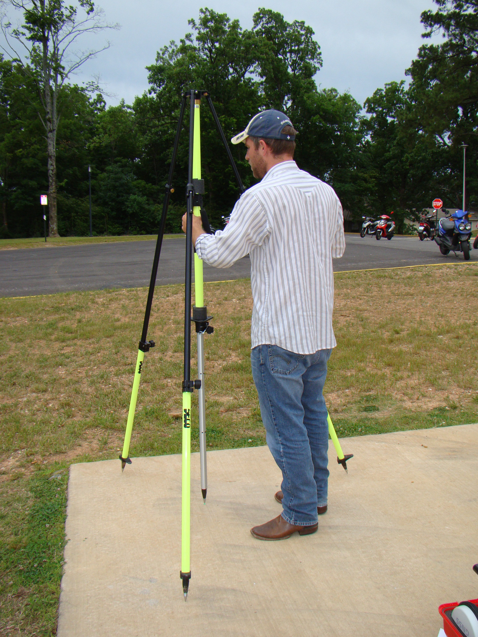
[wptabtitle] Release Tripod Legs[/wptabtitle]

[wptabcontent]

Two of the side legs have squeeze clamps at their upper end. To release them from the tripod base, squeeze the clamp and lift the leg up so that the tip clears the base. Angle the leg away from the tripod body and flip the lever to release the lower clamp on the leg. Extend the lower portion of the leg all the way, and then lock the clamp again.

[wptabtitle] Extend Legs[/wptabtitle]

[wptabcontent]

Finally, use the squeeze clamp to extend the leg all the way to the ground, forming a stable angle with the center pole. Repeat this operation with the second leg that also has a squeeze clamp.

[wptabtitle] Secure Legs[/wptabtitle]

[wptabcontent]

The third leg is different; instead of a squeeze clamp, it uses a thumb screw to tighten the upper section.

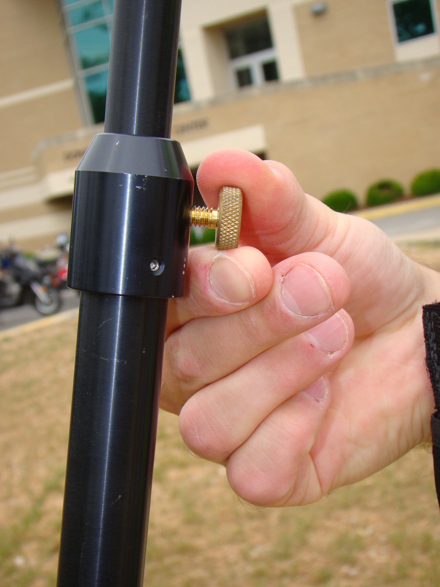
Loosen this thumbscrew, and then extend the leg and place its tip as you did on the other two legs. Be sure to leave the thumbscrew loose. At this time, if your are on soft ground, you should use your foot to push each of the three legs (not the center pole) into the ground.

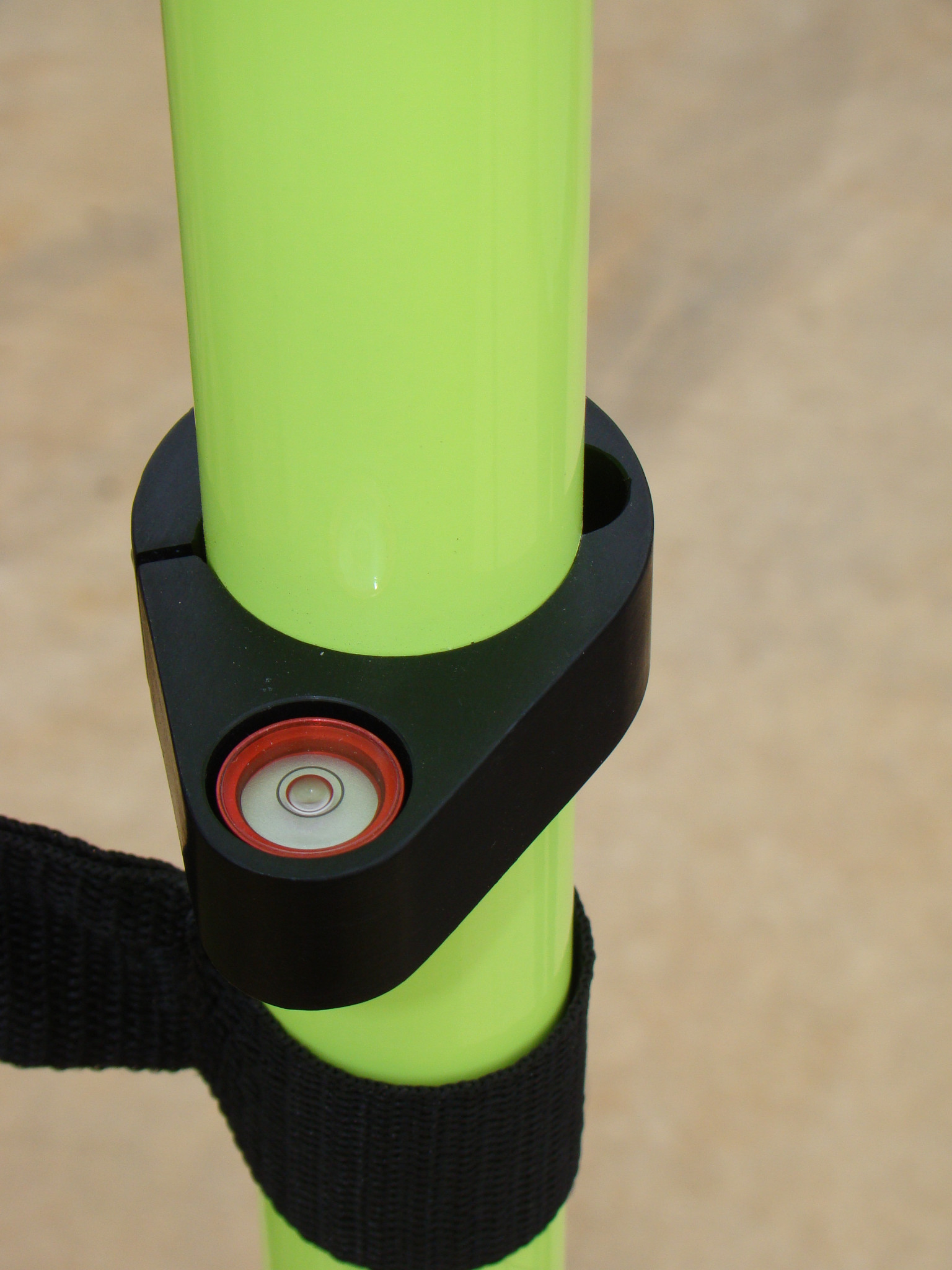
[wptabtitle] Level Tripod[/wptabtitle]

[wptabcontent]

The tripod must be completely level to get an accurate measurement. Locate the bubble level mounted on the side of the tripod. Place a hand on each of the squeeze clamps, squeeze them to release their lock, and very carefully push or pull to align the air bubble in the level within the inner marked circle.

When you have the tripod level, release both of the squeeze clamps, and check your level again. If it is still level, lock the thumbscrew on the third leg and you are finished with the tripod.

[/wptabs]

Posted in GPS, Hardware, Leica GS15 Receiver, Setup Operations, Uncategorized

PhotoScan – Building Geometry & Texture for Photogrammetry

This post will show you how to build the geometry and texture for your 3D model and how to export it for use in ArcGIS.
Hint: You can click on any image to see a larger version.

[wptabs mode=”vertical”] [wptabtitle] Rebuild Geometry[/wptabtitle]
[wptabcontent]After the model is georeferenced, rebuild geometry at the desired resolution. Photoscan produces very high poly-count models, so we like to build two models, a high resolution one for archiving and measurements and a lower resolution one for import into ArcGIS for visualization and general reference. Keeping the polycount low (circa 100,000 faces) in the ArcGIS database helps conserve space and speeds up loading time on complicated scenes with multiple models. To make sure the lower poly-count model looks good, we build the textures using the high poly-count model and apply them to the lower poly-count model.

So… Select ‘Workflow’ and ‘Build Geometry’ from the main menu as before. Then select ‘Workflow’ and ‘Build Texture’.

[/wptabcontent]

[wptabtitle]Decimate the model[/wptabtitle]

[wptabcontent]Under ‘Tools’ in the main menu you can select ‘Decimate’ and set the desired poly-count for the model. The decimated model will likely have a smoother appearance when rendered based on vertex color, but will appear similar to the higher poly-count model once the texture is applied.

[/wptabcontent]

[wptabtitle]Export the model[/wptabtitle]
[wptabcontent] Export the models and save them as collada files (.dae) for import into ArcGIS. You may select a different format for archiving, depending on your project’s system. Choose ‘File’ and ‘Export Model’ from the main menu.

[/wptabcontent]

[wptabtitle] Continue to…[/wptabtitle]

Continue to Photoscan to ArcGIS

[wptabcontent]

[/wptabs]

Posted in Workflow

PhotoScan – Basic Processing for Photogrammetry

This series will show you how to create 3d models from photographs using Agisoft Photoscan and Esri ArcGIS.
Hint: You can click on any image to see a larger version.

Many archaeological projects now use photogrammetric modeling to record stratigraphic units and other features during the course of excavation. In another post we discussed bringing photogrammetric or laserscanning derived models into a GIS in situations where you don’t have precise georeferencing information for the model. In this post we will demonstrate how to use bring a photogrammetric model for which georeferenced coordinates are available, using Agisoft’s Photoscan Pro and ArcGIS.

[wptabs mode=”vertical”] [wptabtitle] Load Photos[/wptabtitle] [wptabcontent]Begin by adding the photos used to create the model to an empty project in Photoscan.

[/wptabcontent]

[wptabtitle] Align Photos[/wptabtitle] [wptabcontent]Following the Photoscan Workflow, next align the images. From the menu at the top choose ‘Workflow’>’Align Images’. A popup box will appear where you can input the alignment parameters. We recommend selecting ‘High’ for the accuracy and ‘Generic’ for the pair pre-selection for most convergent photogrammetry projects.

[/wptabcontent]

[wptabtitle] A choice[/wptabtitle] [wptabcontent]At this point there are two approaches to adding the georeferenced points to the project. You can place the points directly on each image and then perform the bundle adjustment, or you can build geometry and then place the points on the 3d model, which will automatically place points on each image, after which you can adjust their positions. We normally follow the second approach, especially for projects where there are a large number of photos.
[/wptabcontent]

[wptabtitle]Build Geometry[/wptabtitle]
[wptabcontent]Under ‘Workflow’ in the main menu, select ‘Build Geometry’. At this point we don’t need to build an uber-high resolution model, because this version of the model is just going to be used to place the markers for the georeferenced points. A higher resolution model can be built later in the process if desired. Therefore either ‘Low’ or ‘Medium’ are good choices for the model resolution, and all other parameters may be left as the defaults. Here we have selected ‘Medium’ as the resolution.

[/wptabcontent]

[wptabtitle]Get the georeferenced points[/wptabtitle]
[wptabcontent]When the photos for this model were taken, targets were places around the feature (highly technical coca-cola bottle caps!) and surveyed using a total station. These surveyed targets are used to georeference the entire model. In this project all surveyed and georeferenced points are stored in an ArcGIS geodatabase. The points for this model are selected using a definition query and exported from ArcGIS.

[/wptabcontent]

[wptabtitle]Add the georeferenced points[/wptabtitle]
[wptabcontent]On the left you have two tabbed menus, ‘Workspace’ and ‘Ground Control’. Switch to the the ‘Ground Control’ menu. Using the ‘Place Markers’ tool from the top menu, place a point on each surveyed target. Enter the corresponding coordinates from the surveyed points through the ‘Ground Control’ menu. Be careful to check that the northing, easting and height fields map correctly when importing points into Photoscan, as they may be in a different order than in ArcGIS.

[/wptabcontent]

[wptabtitle]Local coordinates and projections[/wptabtitle]
[wptabcontent] In practice we have found that many 3d modelling programs don’t like it if the model is too far from the world’s origin. This means that while Photoscan provides the tools for you to store your model in a real world coordinate system, and this works nicely for producing models as DEMs, you will need to use a local coordinate system if you want to produce models as .obj, .dae, .x3d or other modeling formats and work with them in editing programs like Rapidform or Meshlab. If your surveyed coordinates involve large numbers e.g. UTM coordinates, we suggest creating a local grid by splicing the coordinates so they only have 3-4 pre decimal digits. [/wptabcontent]

[wptabtitle]Bundle Adjust – Another Choice[/wptabtitle]
[wptabcontent]After all the points have been placed select all of them (checks on). If you believe the accuracy of the model is at least three time greater than the accuracy of the ground control survey you may select ‘update’ and the model will be block shifted to the ground control coordinates. If you believe the accuracy of the ground control survey is near to or greater than the accuracy of the model, you should include these points in your bundle adjustment to increase the overall accuracy of the model. To do this select ‘optimize’ from the ‘Ground Control’ menu after you have added the points. After the process runs, you can check the errors on each point. They should be less than 20 pixels. If the errors are high, you can attempt to improve the solution by turning off the surveyed points with the highest error, removing poorly referenced photos from the project, or adjusting the location of the surveyed points in individual images. After adjustments are made select ‘update’ and then ‘optimize’ again to reprocess the model.

[/wptabcontent]

[wptabtitle] Continue to…[/wptabtitle]

Continue to PhotoScan – Building Geometry & Texture for Photogrammetry

[wptabcontent]

This document is under development…Please check back soon

Posted in Uncategorized

Acquire External Control with Trimble 5700/5800

This page is a guide for acquiring external control for close range photogrammetry using Trimble survey grade GPS.
Hint: You can click on any image to see a larger version.

[wptabs mode=”vertical”]

[wptabtitle] Prepare for Survey[/wptabtitle]

[wptabcontent]

Begin metadata process
1. Choose a method for documenting the project (e.g. notebook, laptop)
2. Fill in known metadata items (e.g. project name, date of survey, site location, etc.)
3. Create a sketch map of the area (by hand or available GIS/maps)
Choose and prepare equipment
1. Decide what equipment will best suite the project
2. Test equipment for proper functioning and charge/replace batteries

[/wptabcontent]

[wptabtitle] Equipment Setup[/wptabtitle]

[wptabcontent]

Base station
1. Setup and level the fixed height tripod over the point of your choice
2. Attach the yellow cable to the Zephyr antenna
3. Place the Zephyr antenna on top using the brass fixture and tighten screw
4. Attach the yellow cable to the 5700 receiver
5. Attach the external battery to the 5700 receiver (if using)
6. Attach the data cable to the TSCe Controller and turn the controller on
7. Create a new file and begin the survey
8. Disconnect TSCe Controller
Rover
1. Put two batteries in the 5800
2. Attach the 5800 to the bipod
3. Attach TSCe Controller to bipod using controller mount
4. Connect data cable to 5800 and TSCe Controller
5. Turn on the 5800 and controller
6. Create a new project file (to be used all day)

[/wptabcontent]
[wptabtitle] Collecting Points[/wptabtitle]

[wptabcontent]

Have documentation materials ready
1. As you collect points, follow ADS standards
Base station
1. Once started, the base station will continually collect positions until stopped
2. When you’re ready to stop it, connect the TSCe controller to the receiver and end the survey
Rover
1. When you arrive at a point you want to record, set the bipod up and level it over the point
2. Using the controller, create a new point and name it
3. Start collecting positions for the point and let it continue for the appropriate amount of time
4. Stop collection when time is reached and move to next position

[/wptabcontent]
[wptabtitle] Data Processing[/wptabtitle]

[wptabcontent]

Have documentation materials ready
1. As you process the data, follow ADS standards
Transfer data
1. Use Trimble Geomatics Office (TGO) to transfer data files from the TSCe Controller and the 5700 receiver to the computer
Calculate baselines
1. Use TGO to calculate baselines between base station and rover points
2. Apply adjustment and export points

[/wptabcontent]
[/wptabs]

Posted in GPS, Hardware, Setup Operations, Setup Operations | Tagged Centimeter, Data Collection, GPS, GPS model 5700, GPS model 5800, GPS Pathfinder Office, Photogrammetry, Sub-meter, Trimble GPS, Workflow

Pathfinder Office "How To" Guide

This page demonstrates how to create a data dictionary in Pathfinder Office, transfer it to a GPS receiver, transfer data from the receiver to Pathfinder Office, differentially correct the data, and export it for use in ArcGIS.
Hint: You can click on any image to see a larger version.

[wptabs mode=”vertical”]

[wptabtitle] Create Data Dictionary[/wptabtitle]

[wptabcontent]

A data dictionary makes GPS mapping easier by allowing you to predefine and organize point, line, and area features and their associated attributes. The feature and attribute examples in this guide are used to demonstrate how to use the Data Dictionary Editor in Pathfinder Office and to demonstrate the types of parameters that can be set.

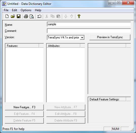
To begin, open Pathfinder Office and create a new project. Make sure that the outputs are going to your preferred drive and file location. Click on “Utilities” located along the menu bar. Choose “Data Dictionary Editor” and provide an appropriate title for your data dictionary. For the purposes of this guide, the name of the data dictionary is “sample.”

Next, you may define the features to be included in the data dictionary. The features will belong to one of the following feature classes: point, line, or area.

[wptabtitle] Point Feature[/wptabtitle]

[wptabcontent]

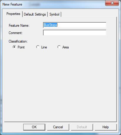
Create a point feature by selecting “New Feature.” The feature classification will be “point.” In this example, the point features that we want to map are bus stops. So, the feature name will be “BusStops.”

Under the “Default Settings” tab, choose a logging interval of 1 second and set minimum positions to 120. The logging interval determines how often a GPS position is logged. Acquiring at least 120 positions per point feature will ensure better accuracy (the positions are averaged to determine location). During data collection, the receiver will give a warning message if you attempt to stop logging the feature before 120 positions have been recorded. When finished with the parameters on these tabs, press OK.

To set attribute information to be recorded with the mapped feature, select “New Attribute.” A window will open allowing you to select the type of attribute you wish to define. In this example we would like to name the bus route. Therefore the attribute type will be text. Choose “Text” and enter “RouteName” in the Name field. Note that the Length field is important because the value specifies the number of characters that can be entered when defining the attribute (be sure that the value is sufficient for the length needed). In the New Attribute dialog box, there is an option to require field entry upon creation. Selecting this option will ensure that you enter the attribute upon creation of the feature during data collection. Click OK to save the attribute – you will see it appear in the Attributes window in the Data Dictionary Editor.

You may now define another attribute type. For example, we may wish to record how many people were at the bus stop at the date and time that the feature was mapped. In this case, we want to select both “Date” and “Time” from the New Attribute Type window. To record the number of people, a numeric attribute is needed. After choosing “Numeric,” enter “# of people” in the name field. Note that a minimum and maximum value should be set for the number of people possible (for example, a minimum of 0 and max of 50). You must also set a default number that is within the range of the minimum and maximum values. If you do not update this attribute during data collection, the default value will be used.

Finish setting all of the desired attributes for the point feature and then close the New Attribute Type dialog box before creating the next feature in the data dictionary.

[wptabtitle] Line Feature[/wptabtitle]

[wptabcontent]

Create a line feature by selecting “New Feature.” The feature classification will be “line.” In this example, the line features that we want to map are sidewalks. So, the feature name will be “Sidewalks.”

Under the Default Settings tab, choose a logging interval of 5 seconds. Logging one position every 5 seconds should be sufficient when collecting a feature while walking. You may want to experiment with different values here to test the accuracy of your results. When finished with the parameters on these tabs, press OK.

To set attribute information to be recorded with the mapped feature, select “New Attribute.” A window will open allowing you to select the type of attribute you wish to define. In this example we would like to specify the type of material that the sidewalk is composed of (cement, asphalt, or unpaved). The easiest way to record this attribute type is with a menu. Choose “Menu” and enter “Material” in the Name field. Under “Menu Attribute Values,” press the “New…” button. Type “cement” in the Attribute Value field and press “Add.” Cement will appear under “Menu Attribute Values” and the New Attribute Value – Menu Item window will clear. Next type “asphalt” in the Attribute Value field and press “Add.” Finally “unpaved” may be entered in the Attribute Value field. Press “Add” and then close the New Attribute Value – Menu Item window. To require this attribute to be entered upon creation of the feature, select the “Required” option under Field Entry. Selecting this option will ensure that you enter the attribute upon creation of the feature during data collection.

Press OK to save the attribute before defining the next feature.

[wptabtitle] Area Feature[/wptabtitle]

[wptabcontent]

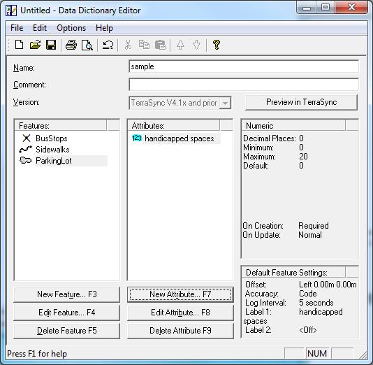
Create an area feature by selecting “New Feature.” The feature classification will be “area.” In this example, the area features that we want to map are parking lots. So, the feature name will be “ParkingLot.” Under the Default Settings tab, choose a logging interval of 5 seconds. Logging one position every 5 seconds should be sufficient when collecting a feature while walking. You may want to experiment with different values here to test the accuracy of your results. When finished with the parameters on these tabs, press OK.

To set attribute information to be recorded with the mapped feature, select “New Attribute.” A window will open allowing you to select the type of attribute you wish to define. In this example we would like to record the number of handicapped parking spaces in the parking lot. To record the number of handicapped parking spaces, a numeric attribute is needed. After choosing “Numeric,” enter “handicapped spaces” in the name field. Note that a minimum and maximum value should be set for the possible number of handicapped parking spaces(for example, a minimum of 0 and max of 20). You must also set a default number that is within the range of the minimum and maximum values. If you do not update this attribute during data collection, the default value will be used.

Finish setting all of the desired attributes for the area feature and then close the New Attribute Type dialog box.

[wptabtitle] Save Data Dictionary[/wptabtitle]

[wptabcontent]

To save the data dictionary, choose “File” in the menu bar of the Data Dictionary Editor and select “Save As.” Be sure to save the .ddf (data dictionary file) on your preferred drive and file location. The Data Dictionary Editor may then be closed. You are now ready to transfer the data dictionary to the GPS receiver.

[wptabtitle] Transfer .ddf to GPS Receiver[/wptabtitle]

[wptabcontent]

Open either Active Sync (Windows XP) or Windows Mobile Devices (Windows 7) on the computer. Turn on the GPS receiver and then plug it into a USB port on the computer. It should automatically connect to the computer. It is recommended to NOT sync the receiver with the computer.

Open Pathfinder Office (PFO) while the GPS receiver is connected to the computer. In PFO, go to Utilities > Data Transfer > select the “Send” tab > select “Add” > Data Dictionary > the file defaults to the last .ddf that was created (if not – browse to where the .ddf is located) > select the .ddf and click “Open.”

Under Files to Send, select the file by clicking it (it will become highlighted) > Transfer All

Once the data dictionary has been successfully transferred, you may close out of PFO.

You are now ready for data collection!

[wptabtitle] Transfer Data from Receiver to PFO[/wptabtitle]

[wptabcontent]

After data collection, transfer the data from the receiver to Pathfinder Office (PFO) by first connecting the GPS receiver to the computer. Open Pathfinder Office and then open the project.

Within PFO, choose Utilities > Data Transfer > Add > Data File. Select the files to transfer and choose Open. Highlight the file(s) and choose Transfer all. Close the data transfer box once the file(s) successfully transferred.

View your file by opening the Map (View > Map) and then choosing File > Open > and then selecting the file.

At this point, you may wish to improve the accuracy of the data through differentially correction.

[wptabtitle] Differential Correction[/wptabtitle]

[wptabcontent]

To differentially correct your features, complete the following steps:

Open the data in PFO > go to Utilities > Differential Correction > Next > Auto Carrier and Code Proc > Next > Output Corrected and Uncorrected > Use smart auto filtering > Re-correct real-time positions > OK > Next > Select your nearest Base Provider.

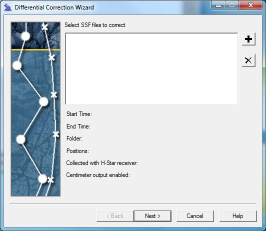
A report showing the accuracy of the results will be generated after differential correction has been completed. The differentially corrected data may be exported for use in other programs including ArcGIS.

[wptabtitle] Export Data for use in ArcGIS[/wptabtitle]

[wptabcontent]

To export the data from PFO, select Utilities > Export. Be sure the Output Folder is set to where you want the output file located (and be sure to remember the file path).

Export as Sample ESRI Shapefle Setup > OK.

Make sure that you are also exporting the uncorrected positions (select “Properties…” > select the “Position Filter” tab > check the box next to “Uncorrected” under Include Positions that Are > OK). This will ensure that positions that have not been corrected will also be exported.

Continue with the export even if no ESRI projection file has been found.

PFO can be closed once file has been successfully exported.

[/wptabs]

This document is under development…Please check back soon

Posted in Uncategorized

Using TerraSync: The Basics

This page will show you how to configure a GPS receiver with TerraSync and how to set and navigate to waypoints.
Hint: You can click on any image to see a larger version.

This guide is written for use with TerraSync v.5.41. The instructions vary only slightly for earlier versions of the software. Reference the tab titled, Menu Hierarchy to become familiar with the terminology used in the instructions.

[wptabs mode=”vertical”]

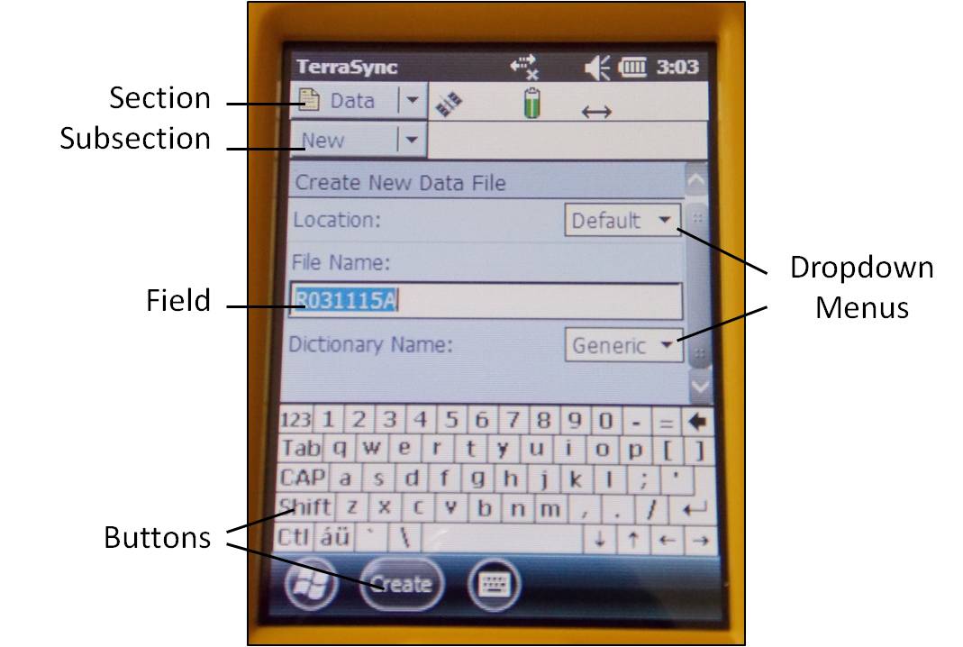
[wptabtitle] Menu Hierarchy[/wptabtitle]

[wptabcontent]

The TerraSync menu system hierarchy is as follows: sections, subsections, buttons, and fields (click on image below). The information provided in the tabs throughout this series will utilize this terminology.

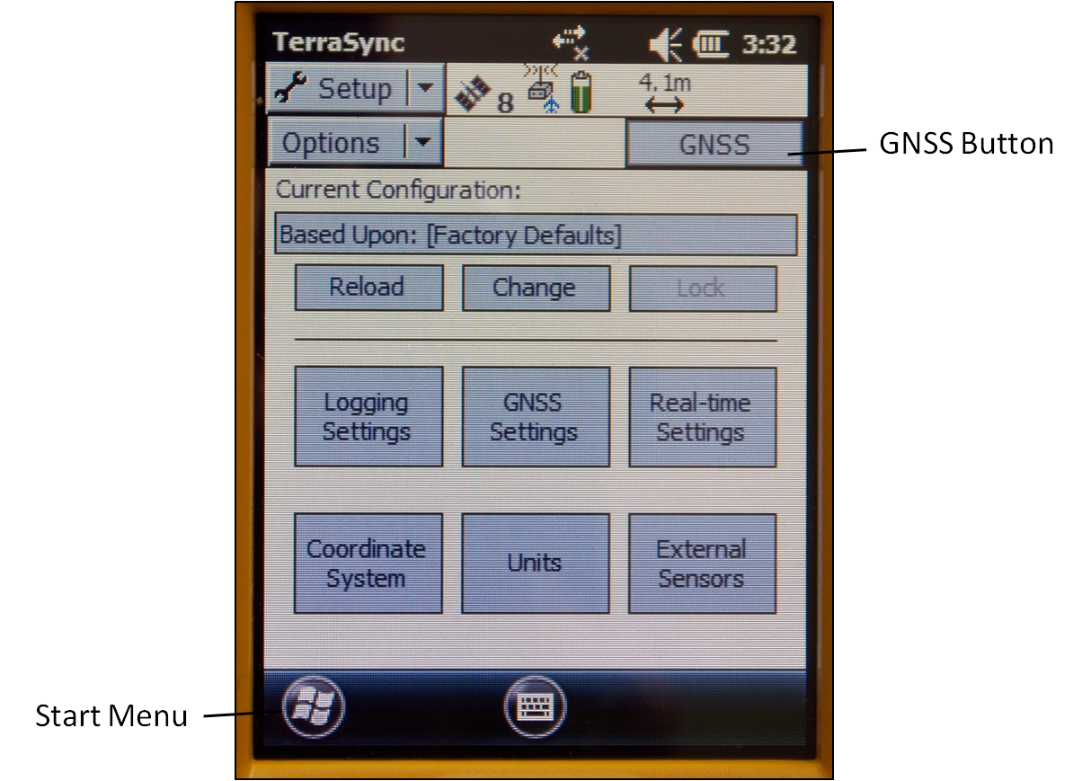
[wptabtitle] Start Terra Sync and Connect to GNSS[/wptabtitle]

[wptabcontent]

Turn on the receiver by pressing the power button. Start TerraSync by opening the Start menu and selecting TerraSync from the menu options. In order to receive information from GNSS satellites, the GPS unit must be connected to the GNSS receiver. To connect to the GNSS receiver, go to the Setup section. Either expand the Options dropdown menu and choose “Connect to GNSS” or press the GNSS button in the upper-right of the screen.

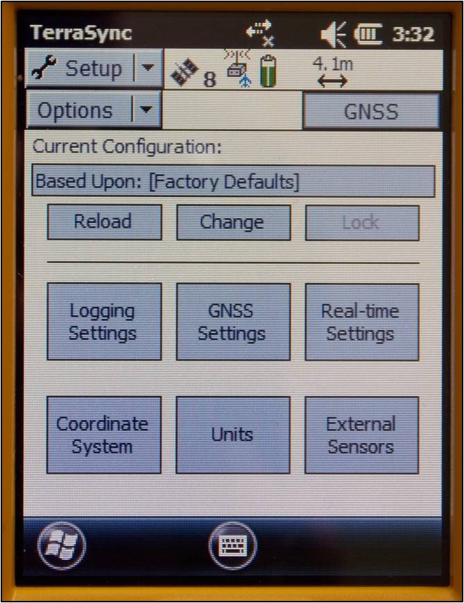
[wptabtitle] Configure GNSS Settings[/wptabtitle]

[wptabcontent]

There are a variety of ways to configure the receiver for data collection under the Setup section in TerraSync. Open each of the six menus to verify that the parameters are set to the desired values. The following are a few parameters to be aware of:

Antenna Settings (under Logging Settings): If you are holding the receiver during data collection and not using an external antenna, you may set the antenna height to 1 meter (which is approximately the height of the receiver above the ground) and choose “Internal” under the Type dropdown menu. When using an external antenna, set the antenna height to the height of the tripod (or whatever height the antenna will be from the ground) and remember to choose the appropriate antenna from the Type dropdown menu.

Real-time Settings: Generally we set Choice 1 to Integrated SBAS, which provides corrections in real-time when a SBAS satellite is available. Set Choice 2 to Use Uncorrected GNSS. If Wait for Real-time is selected, only positions that have been differentially corrected will be used (meaning you may not be able to collect a position unless the receiver is able to make a real-time correction).

Coordinate System: Typically we use Latitude/Longitude with the WGS 1984 datum. However, there may be instances in which you will want to change the coordinate system.

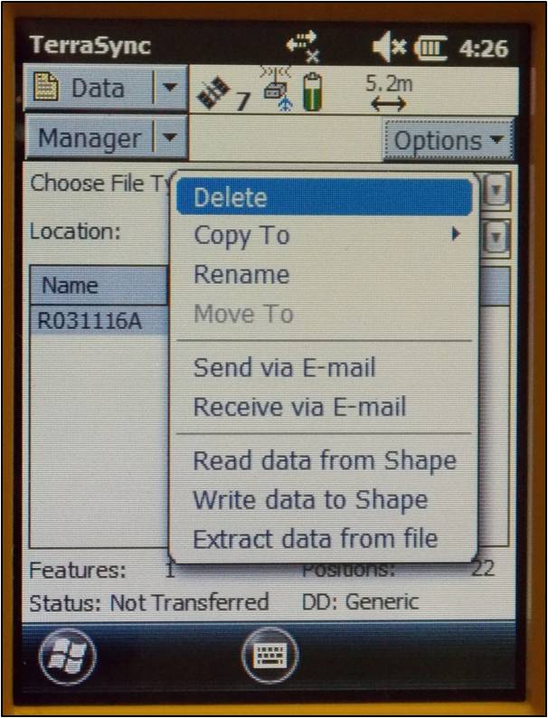
[wptabtitle] Deleting Data[/wptabtitle]

[wptabcontent]

To delete data from the receiver, open the Data section and File Manager subsection. Expand the Choose File Type dropdown menu to select the type of file to delete. Note: It is recommended not to delete Geoid files unless necessary. Select the file you wish to delete by tapping on it (it will be highlighted in blue when it is selected). Press the Options button and choose Delete.

[wptabtitle] Setting Waypoints[/wptabtitle]

[wptabcontent]

To set waypoints on the receiver, open the Navigate section and Waypoint subsection. Tap the New button at the bottom of the screen (note: if a waypoint file is currently open, you must close it before creating a new file – Options > Close File). Give the file a name (or leave the default name) and tap Done. Expand the Options dropdown menu and choose New.

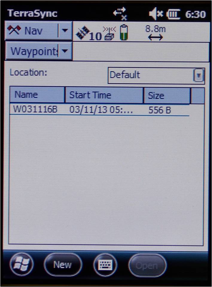
If you have known coordinates to which you would like to navigate, you may manually enter the coordinates. If you wish to mark a GPS position as a waypoint, expand the Create From dropdown menu and choose GNSS. This option auto-fills the coordinates based on the current GPS position.

[wptabtitle] Navigating to a Waypoint[/wptabtitle]

[wptabcontent]

To use the receiver to navigate to an established waypoint, open the Navigate section and Waypoint subsection. Select the waypoint you want to navigate to by tapping the box next to the waypoint (a check will appear in the box). Expand the Options dropdown menu and select Set Nav Target.

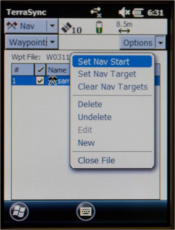
Open the Navigate subsection. You should see the name of the waypoint listed at the top of the screen just below the satellite icon. You are now ready to begin navigating. You must start moving in order for the receiver to become oriented in space and give you directions. It doesn’t matter which direction, just start moving. You may adjust the navigation settings by expanding the Options dropdown menu and selecting Navigation Options.

After reaching a waypoint, you may expand the Options dropdown menu while in the Navigate subsection and choose Goto Next Unvisited Waypoint. Alternatively, you may clear the waypoint by opening the Waypoints subsection, expanding the Options dropdown menu and selecting Clear Nav Target. You may then set your next navigation target.

[/wptabs]

Posted in GPS, Setup Operations, Setup Operations, Trimble GeoExplorer, Trimble Juno, Uncategorized | Tagged GeoExplorer, Juno, terrasync, waypoint

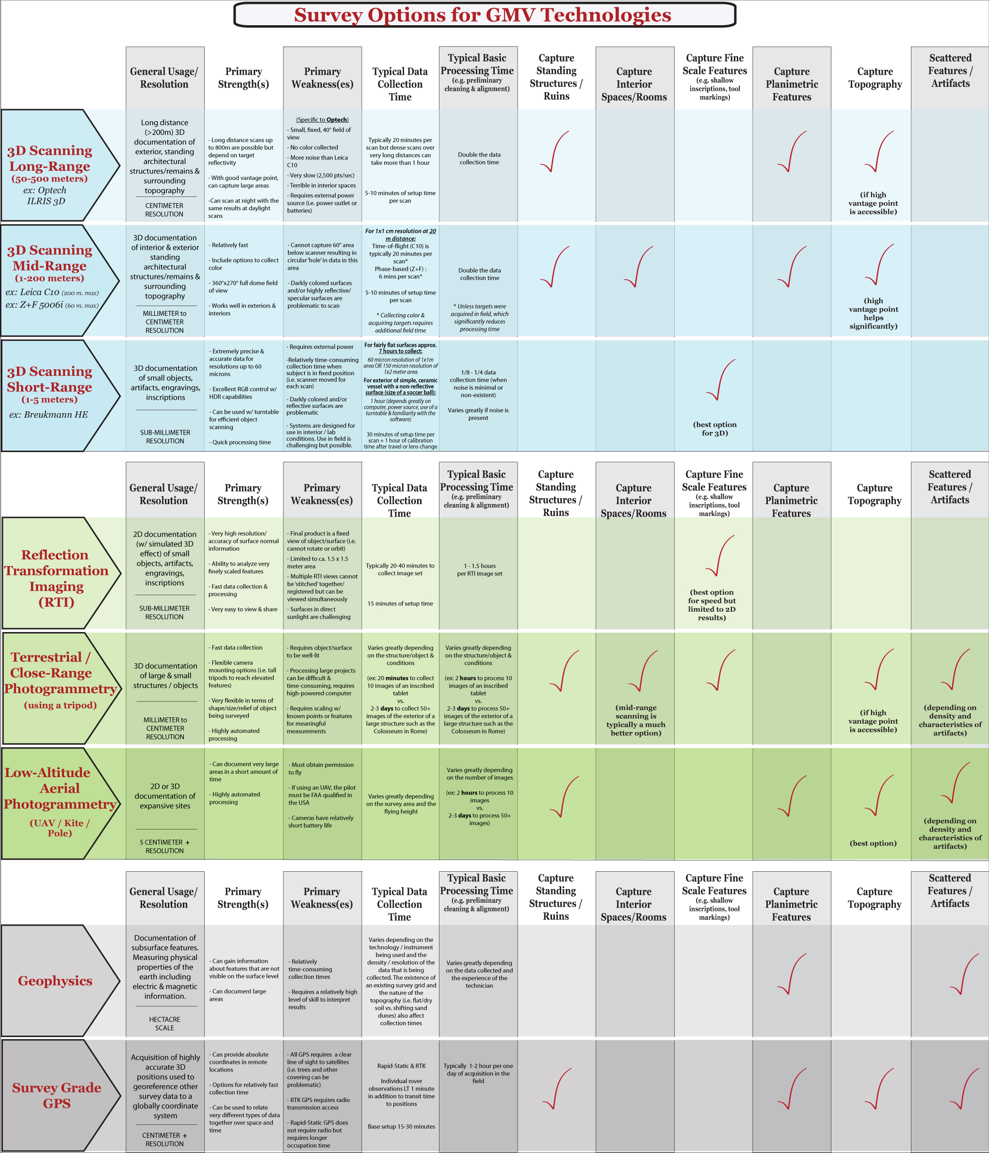
Survey Options for GMV Technologies – Summary Table

Click on the image below to activate the interactive guide. The table summarizes the technologies referenced on the GMV, their typical applications and properties as experienced in the projects and workflows within this site.

Posted in Uncategorized

Leica GS15 RTK: Configuring a GS15 Receiver as a Rover

This page will show you how to use a Leica CS15 to configure a GS15 to be a rover for an RTK GPS survey.
Hint: You can click on any image to see a larger version.

[wptabs mode=”vertical”]

[wptabtitle] Power up the GS15 Rover[/wptabtitle]

[wptabcontent]

Power on the second GS15 receiver – this will be the Rover – and wait for it to start up, then make sure the RTK Rover (arrow pointing down) LED lights up green.

[/wptabcontent]

[wptabtitle] Configure CS15 for Rover[/wptabtitle]

[wptabcontent]

You should probably be at the Base Menu and “Go to Work” (on right) If not you may be in the Job: “Your name” menu and the “Go to Work” button has “Survey & State Points” and “Start Base” as shown below on left.

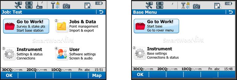
If you have the left screen (Job: TEST –or whatever you named the job– and “Start Base Station”) you simply need to click on the Go to work” and then select “Go to Base menu” – that will take you to the situation shown on the RIGHT image.

[/wptabcontent]

[wptabtitle] Go to Rover Menu[/wptabtitle]

[wptabcontent]

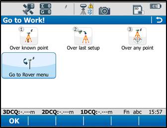
From the main menu, tap “Go to Work!” then “Go to Rover menu.” The unit will take a few moments to connect to the GS15 rover unit. Note: Tap “No” if the Bluetooth connection Warning appears.

[/wptabcontent]

[wptabtitle] Satellite Tracking Settings[/wptabtitle]

[wptabcontent]

Once in the rover menu, tap “Instrument” → “GPS Settings” → “Satellite Tracking.”

In the Tracking tab, make sure that GPS L5 and Glonass are checked on. Also make sure “Show message & audio warning when loss of lock occurs” is checked. The Advanced tab allows you to define other options for the job, and it is appropriate to use the system default settings. Tap OK when finished.

[/wptabcontent]

[wptabtitle]Quality Control Settings[/wptabtitle]

[wptabcontent]

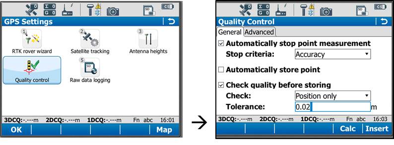
On the rover main menu, tap “Instrument” → “GPS Settings” → “Quality Control.” Here you can define your specifications for RTK point collection with the rover unit. For high precision survey work, it is a good idea to set the tolerance to less than or equal to 2 centimeters, as this will prevent the logging of an RTK point with error greater than this threshold. Tap OK to return to the main menu when finished.

[/wptabcontent]

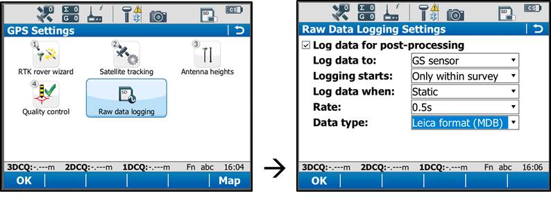
[wptabtitle]Raw Data Logging Settings[/wptabtitle]

[wptabcontent]

On the rover main menu, tap “Instrument” → “GPS Settings” → “Raw Data Logging.” Be sure the box for “Log data for post processing is checked on, then choose where you would like the data to be logged to. We can log to either the receiver’s (GS15) SD card or the controller’s (CS15) SD card. Make sure the controller option has been selected from the drop down list. The remaining options are up to the user to define. Tap OK when done.

[/wptabcontent]

[wptabtitle]RTK Rover Settings: General Tab[/wptabtitle]

[wptabcontent]

On the rover main menu, tap “Instrument” → “Connections” → “All other connections.” On the GS connections tab, tap the RTK Rover connection to highlight it, and then tap “Edit” at the bottom of the screen.

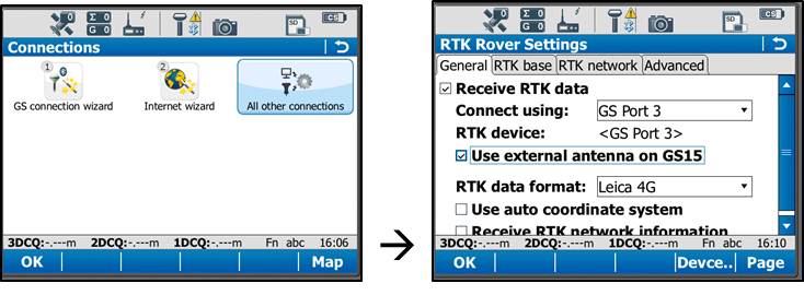
On the General tab, make sure the “Receive RTK data” box is checked on, then verify the following settings:

Connect Using: GS Port 3

RTK Device: Pac Crest ADL (note: different than shown in image above)

(Check on “Use external antenna on GS15”)

RTK Data format: Leica 4G

(Leave the remaining 2 boxes unchecked)

[/wptabcontent]

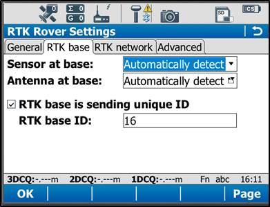
[wptabtitle]RTK Rover Settings: RTK Base Tab[/wptabtitle]

[wptabcontent]

On the RTK base tab, verify the following settings:

Sensor at base: Automatically Detect

Antenna at base: Automatically Detect

(Check on “RTK base is sending unique ID”)

RTK base ID: 16

Tap OK in the bottom left corner. Tap OK if a warning about the antenna pops up. Now tap “Cntrl” at the bottom of the screen. Ensure the following settings are present:

Radio Type: Pac Crest ADL

Channel: 1

Actual frequency: 461.0250 MHz

Tap OK. Tap OK again to return to the main menu.

[/wptabcontent]

[wptabtitle]Finish Setup[/wptabtitle]

[wptabcontent]

At this point the equipment is set up. Now you can begin to take RTK points. You can begin your work or you can power down the CS15 by holding the power button down until the power options menu appears, and select “Turn off.” You can also power down the GS15 receiver by holding the power button until the LEDs flash red.

[/wptabcontent]

[wptabtitle]Continue To…[/wptabtitle]

[wptabcontent]

Continue to “Leica GS15: Tripod Setup”

[/wptabcontent]

[/wptabs]

Posted in GPS, Hardware, Leica CS 15 Controller, Leica GS15 Receiver, Setup Operations, Setup Operations

Leica GS15 RTK: Configuring a GS15 Receiver as a Base

This page will show you how to use a Leica CS15 to configure a GS15 to be a base for an RTK GPS survey.
Hint: You can click on any image to see a larger version.

[wptabs mode=”vertical”]

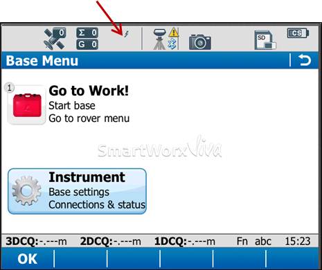
[wptabtitle] Go to Base Menu[/wptabtitle]

[wptabcontent]

Look at the real-time status icon at the top of the CS15 controller screen. If you see a jagged arrow pointed up, the CS15 is in the base menu, where you want to be. If the arrow is pointed down, the CS15 is in the rover menu. To switch to the base menu, tap “Go to Work!” then tap “Go to Base menu.”

[/wptabcontent]

[wptabtitle] Satellite Tracking Settings[/wptabtitle]

[wptabcontent]

Once in the base menu, tap “Instrument” → “Base Settings” → “Satellite Tracking.”

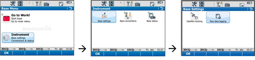
[wptabtitle] Raw Data Logging Settings[/wptabtitle]

[wptabcontent]

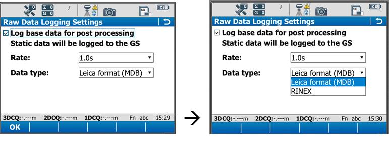
On the base menu, tap “Instrument” → “Base Settings” →”Raw Data Logging.”

Make sure the box is checked for logging base data for post processing. Also confirm that the Data Type is in ‘RINEX’ format. Tap OK.

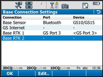
[wptabtitle] Enter Base Connection Settings[/wptabtitle]

[wptabcontent]

Back on the base menu, tap “Instrument” → “Base Connections” → “All other connections.”

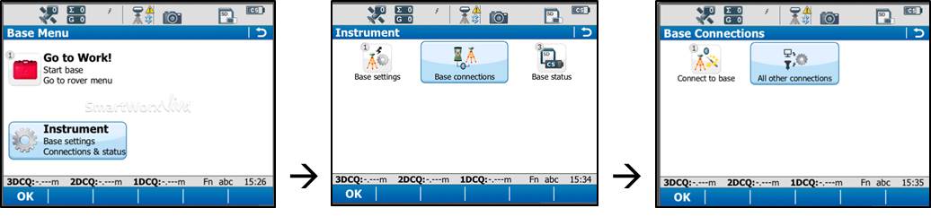
Tap the Base RTK 2 connection to highlight it, and then tap “Edit” at the bottom of the screen.

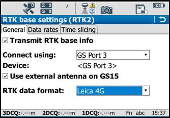
[wptabtitle] Base Connection Settings: General Tab[/wptabtitle]

[wptabcontent]

In the General tab, ensure the box is checked on for “Transmit RTK base info,” then verify the following settings:

Connect Using: GS Port 3

Device: RTK TEST (not as shown on graphic)

RTK Data Format: Leica 4G

Scroll down to see the checkbox for “Use External antenna on GS15.” Generally, you want to use the external antenna, so make sure to check this box.

[wptabtitle] Base Connection Settings: Data Rates Tab[/wptabtitle]

[wptabcontent]

On the Data Rates tab, the default settings are generally fine, but double check the RTK base ID. It should be set to 16, and if it is, it can be left that way. Tap OK in the bottom left corner. Tap OK if a warning about the antenna pops up. Now tap “Cntrl” at the bottom of the screen.

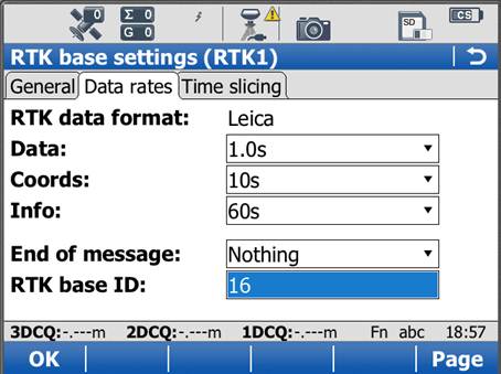
Ensure the following settings are present:

Radio Type: Pac Crest ADL

Channel: 1

Actual frequency: 461.0250 MHz

* The “Actual frequency” will be set at “0.0000MHz” until the GS15 and CS15 are connected.

Tap OK. Tap OK again to return to the main menu.

[wptabtitle] Power up the GS15[/wptabtitle]

[wptabcontent]

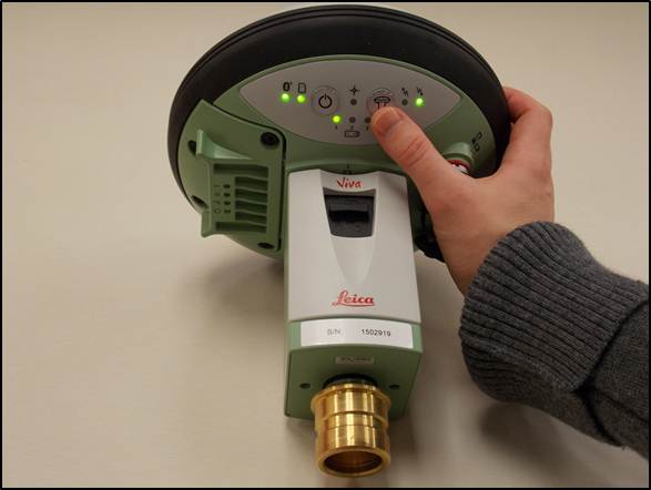
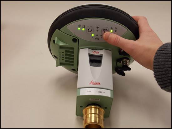
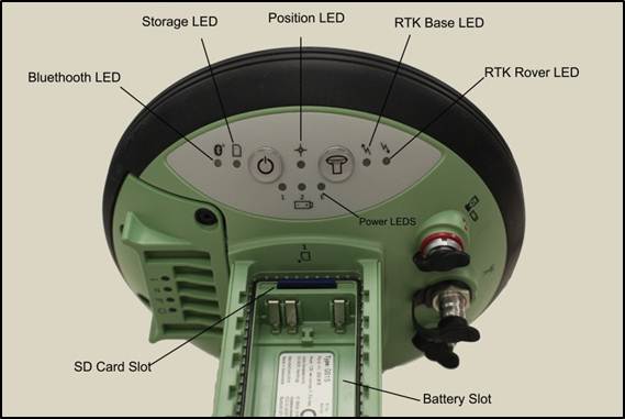
Power up the GS15 receiver that you will be using as a base station (the one that has the SD card in it) by pressing and holding the power button until the 3 LEDs below it light up. Keep the other GS15 that will act as the rover turned off.

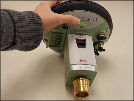
Note: It is important to understand what the buttons, symbols, and LED lights do and/or represent on the GS15 unit. A detailed description of button operation can be found in the Leica “GS10/GS15 User Manual” in section 2.1, pages 20-24. A detailed description of symbols and LEDs can be found in the same manual in section 3.5, pages 64-68. The GS15 is powered down by pressing and holding the power button until the LEDs turn red.

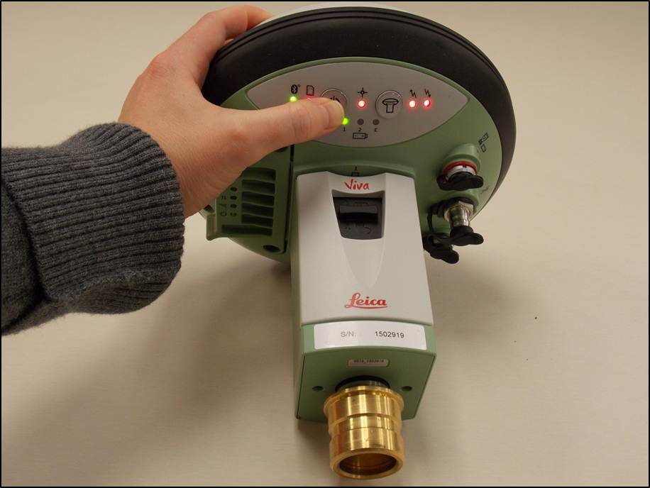
[wptabtitle] Put Base into RTK Mode[/wptabtitle]

[wptabcontent]

Make sure the GS15 unit is in RTK base mode, and set up to broadcast RTK corrections via the radio. To do this, check that the LED beneath the RTK base symbol (arrow pointing up) is lit up green. If the GS15 is in Rover mode (arrow pointing down), you may need to quickly press the function button to change it to Base mode.

[wptabtitle] Connect CS15 to GS15 via Bluetooth[/wptabtitle]

[wptabcontent]

The CS15 should automatically connect to the GS15 unit once it has entered base mode, via Bluetooth. On the CS15, you will see the Bluetooth symbol appear at the top of the screen. On the GS15, the LED beneath the Bluetooth symbol will turn blue.

If the CS15 does not automatically connect with the GS15, you can search for all visible Bluetooth devices. Navigate in the Base menu: ‘Instrument’ → ‘Base connections’ → ‘connect to base’ and click on the “search” button on the bottom of the screen. The “Found Bluetooth devices” screen will appear. The GS15 will be listed under the ‘Name:’ column, named after its serial number. The serial number can be found on a white sticker on the lower side of the GS15, under the battery cover (e.g. “S/N: 1502919”)

You may want to power down the GS15 by pressing and holding the power button until the LEDs turn red if you are in lab configuring but if in field then you can configure the RTK while base is on, BUT – be sure you are connected to the ROVER not the BASE. If you can confirm this by making sure that the Bluetooth connection is the correct serial number.

[wptabtitle] Continue To…[/wptabtitle]

[wptabcontent]

Continue to Part 4 of the series, “Leica GS15 RTK: Configuring a GS15 Receiver as a Rover.”

[/wptabs]

Posted in GPS, Hardware, Leica CS 15 Controller, Leica GS15 Receiver, Setup Operations, Setup Operations

Configuring the CS15 Field Controller

This page will show you how to set the parameters on a Leica CS15 field controller in preparation for GPS survey.
Hint: You can click on any image to see a larger version.

[wptabs mode=”vertical”]

[wptabtitle] Power up the CS15[/wptabtitle]

[wptabcontent]

Power on the CS15 controller by pressing and holding the power button until the screen turns on. The operating system will take a minute to boot up, and will automatically start up the Leica Smartworks interface. Click “No” if the bluetooth connections Warning message pops up.

You may get the Welcome screen. If so, click “Next”.

[/wptabcontent]

[wptabtitle] Choose Survey Instrument[/wptabtitle]

[wptabcontent]

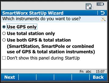
After powering on the controller, you may see the SmartWorx StartUp wizard. Confirm that “GPS Instrument” is selected in the drop-down in the “First Measure with:” menu, or the “use GPS only” radio box.

[wptabtitle]Choose a Job [/wptabtitle]

[wptabcontent]

If these have been turned off by previous users, then the first screen that appears will allow you to “Continue with last used job,” create a “New Job,” or “Choose working Job.” For the purposes of this guide, select “New Job” and tap “Next” in the lower left corner.

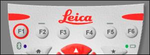
Note that you can also use the “F” key below each entry. So pressing F1 which is below “Next” is the same as using the stylus and clicking on the touch screen. Pressing F6 is the same as pressing the stylus on Back.

[wptabtitle] Set Job Description[/wptabtitle]

[wptabcontent]

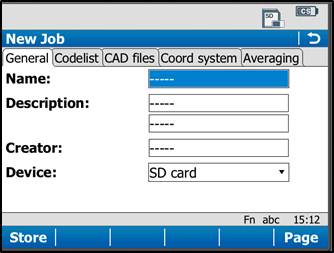
On the General Tab, enter a name for the job, a description, and the name of the person who is creating the job. Be sure to choose “SD Card” for the Device option, as this will result in all the data generated within the job to be saved only to the SD Card.

[wptabtitle]Set Coordinate System[/wptabtitle]

[wptabcontent]

On the “Coord system” tab, be sure the coordinate system is set to “WGS84basic.” If it needs to be changed to this, just tap on the drop down menu, select “WGS84basic,” and tap OK in the lower left corner. You have the ability to create a custom coordinate system if needed (more information can be found in the Leica Technical Manual).

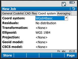
Tap “Store” in the lower left corner to save the job and go to the main menu.

Note: It is beneficial to learn what the icons along the top of the screen represent. For detailed information, see the Leica “Getting Started Guide” section 2.1.2, pages 51-54. Additionally, a brief and simple presentation of the main menu options can be found in the Leica “Getting Started Guide” section 2.1.3, pages 55-57.

[wptabtitle]Continue To…[/wptabtitle]

[wptabcontent]

Continue to Part 3 of the series, “Leica GS15 RTK: Configuring a GS15 Receiver as a Base.”

[/wptabs]

Posted in GPS, Hardware, Leica CS 15 Controller, Leica GS15 Receiver, Setup Operations, Setup Operations

Leica GS15 RTK: Preliminary Setup before Going into the Field

This page will show you the basic instrument components needed for a Leica GS15 RTK GPS survey and will review memory card maintenance.
Hint: You can click on any image to see a larger version.

[wptabs mode=”vertical”]

[wptabtitle] Instrument Components[/wptabtitle]

[wptabcontent]

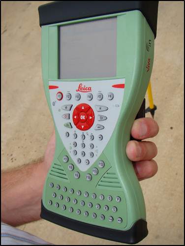
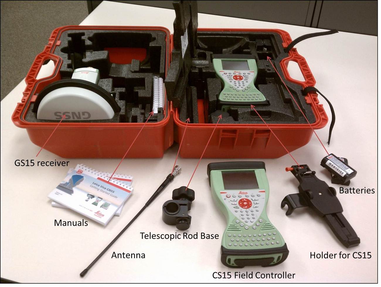
GS15 GNSS receiver (left) and CS15 field controller (right)

[/wptabcontent]

[wptabtitle] Equipment Check List [/wptabtitle]

[wptabcontent]

Minimum equipment and accessories needed (contents of instrument kit):

• GS15 receiver (2)
• CS15 field controller (1)
• Antennas (2 – one for each GS15)
• Holder for CS15 (1)
• Base for telescopic rod (1)
• Batteries
- 5 or more (two for each GS15 and one for the CS15, more depending on length of survey)
- Confirm that batteries are charged
• SD cards
- Enough for each instrument (GS15 and CS15)
- Leica recommends 1GB
- Confirm that cards are not locked via the mechanical locks
• Manuals
- Leica Viva GNSS Getting Started Guide
- Leica GS10/GS15 User Manual
Instruments and their locations in the kit.

[/wptabcontent]

[wptabtitle] Memory Card and Data Maintenance [/wptabtitle]

[wptabcontent]

Make sure memory cards have adequate space for your data needs. The GS15 receivers hold one memory card, which can be accessed in the battery compartment beneath the power button. The CS15 controller also holds a memory card, which can be accessed by using the Phillips screwdriver end of the stylus to loosen the screws on top of the unit. These screws are spring loaded and only take about a half turn to loosen.

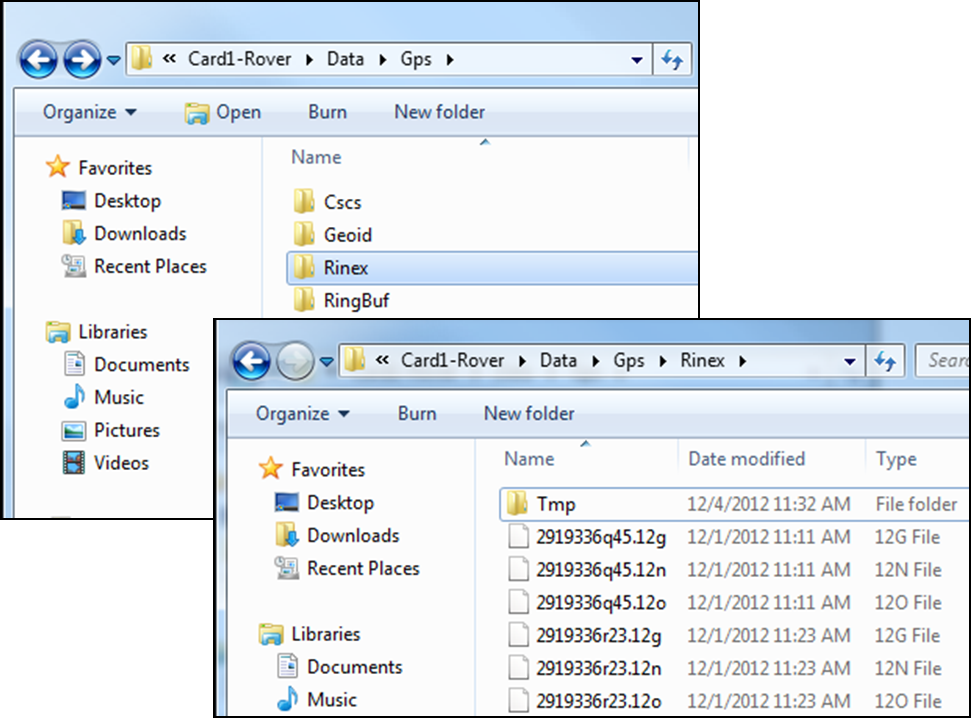
If you are recording Leica data (for example Leica MDX), the files will be found on the SD card in the DBX directory. If you are recording RINEX, the data will be found in DATA> GPS > RINEX.

Note: The raw data files have the following format AAAA_BBBB_CCCCCC with the suffix .m00 for raw Leica data (the suffix .12o is for RINEX). The letters are AAAA = last four numbers of the unit’s serial number BBBB is the date in month and day so 0405 is the fourth month (April) and fifth day. CCCCCC is the hour (two digit 24 hour clock) minute and second. So 5:34 and 21 seconds PM is 173421. This is then followed by .m00 if it is RAW. Note that OPUS will now take Leica RAW as well as RINEX.
*Only delete data from the SD card if it is your own work, or if the original owner has backed up the data. *

[/wptabcontent]

[wptabtitle] Inserting Memory Cards and Batteries [/wptabtitle]

If you plan to record to the controller, place one SD card into the CS15 and secure the top back in place by tightening the screws about a half turn until they lock with the Phillips screwdriver end of the stylus. You do not NEED to record to the controller but it may provide redundancy. Place the other SD card into one of the GS15 receivers. The GS15 that has the memory card will be used as the base station (you may set the rover to write to the controller).

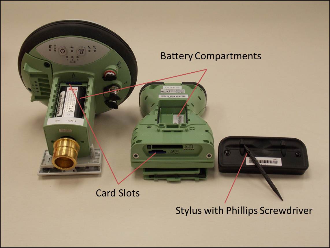
Insert fully charged Lithium Ion batteries into all devices. The GS15 receivers can hold 2 batteries, which are stored below the antenna portion of the unit in the compartments on either side. The battery for the CS15 is located in a compartment on the back. To access this compartment, you will likely have to remove the mounting base first. To do this, slide the red bar to the right in order to unlock the mount. Gently wiggle the mount and pull away from the CS15 to detach it. The battery compartment is now accessible. Replace the mount by popping it back into place and slide the red bar all the way back to left, which locks the mount to the CS15 controller.

[wptabtitle] Continue To… [/wptabtitle]

[wptabcontent]

Continue to Part 2 of the Series, “Leica GS15 RTK: Configuring the CS15 Field Controller.”

[/wptabcontent]

[/wptabs]

Posted in Checklist, Checklist, GPS, GPS Data, Hardware, Leica CS 15 Controller, Leica GS15 Receiver, Setup Operations, Setup Operations, Uncategorized

Evaluating Objectives for Data

This document will introduce you to some of the initial questions that are posed when evaluating the overall objectives for your data as they relate to processing and future use.
Hint: You can click on any image to see a larger version.

[wptabs style=”wpui-alma” mode=”vertical”] [wptabtitle] INTENDED AUDIENCE OF THIS GUIDE [/wptabtitle]

[wptabcontent]

Who will find this guide useful?

The growing number of digital technologies that allow for rapid and accurate documentation of sites and objects that are described on the GMV and within these guides, can acquire substantial amounts of data in a relatively short time in the field. In general, the resulting data are part of a larger data life cycle structure and are acquired with an appreciation of the wide range of possible future uses.

By the time that you are reading this, we assume that you are familiar with the types of data on the GMV and the types of applications and projects in which CAST uses them as outlined on the Using the GMV page and within individual technology sections. You should now also be familiar with the main ideas within the table Survey Options for GMV Technologies. In order to make use of this guide, you need to have a basic to intermediate understanding of these technologies and ideas.

______________________________________________________________

ADDITIONAL RESOURCES : In projects in which the quality and quantity of data to be collected is still being decided, this document is intended to be used in conjunction with the GMV’s Evaluating the Project Scope Document. Ideally, the ultimate destination of the data would be considered in the planning and collection stages. However, whether you making these decisions and collecting the data yourself or not, we hope that considering the objectives in this document will aid you in relating your data to the ‘big picture’.

The Archaeology Data Service / Digital Antiquity Guides to Good Practice provides much more detail about data management while this document attempts to simplify very complex topics for a more generalized understanding.

[/wptabcontent]

[wptabtitle] OBJECTIVE [/wptabtitle] [wptabcontent]

Goal of this Guide

It is critical to note that the topics discussed here focus ONLY on general, basic processing of data that is necessary to make it intelligible to others and ready for an archive. That said, the data acquisition, processing and archiving referenced here are intended to be part of a larger data life cycle structure with an understanding of possible future uses. It is, of course, impossible to anticipate all future uses to which data may be applied but the objectives considered here are designed to obtain well documented and comprehensive data that can be expected to support a broad range of future applications and analyses, within heritage applications and beyond.

The primary objective of this document is to aid users in evaluating overall goals for data and how they relate to maintaining archivable and reusable data by considering :

I. What is the overall life cycle of the data?

II. How is preparing data for archival quality related to the products produced for end ‘consumption’?

II. What types of error are involved with the data?

III. What are your overall goals for data processing? How does the data evolve over each stage of processing from the original data to final files or products that you are hoping to produce?

[/wptabcontent]

[wptabtitle] DATA LIFE CYCLE [/wptabtitle] [wptabcontent]

What is the Life Cycle of Your Data?

A Documentation Perspective : When properly considered, the life cycle of your data begins before any data is collected. The first concept of the data occurs early in project planning when decisions relating to the data, such as file types, naming conventions, and documentation methods, are made. Many projects and the great majority of heritage recordation efforts move directly from the acquisition and creation efforts to development and presentation of a specific set of work products. In general, here, we instead look at digital heritage and urban recordation data with a focus on a documentation perspective that keeps an ongoing life cycle in mind. This perspective involves multiple technologies in which the initial product is data in an archival quality that allows for a variety of end ‘consumption’ – including display, analysis and presentation products that are not covered here.

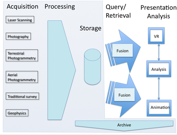
The data life cycle. Shaded portions of the life cycle are the topics of focus in this guide.

Heritage and Modern Environments : It should be noted that, in general, heritage guidelines for documenting these evolving technologies are far more advanced than the standards for projects involving modern environments. As disciplines that deal with modern environments (such as architects, engineers and city planners) become increasingly aware of these technologies and begin utilizing them for building information and daily maintenance/operations objectives, standards for these applications will continue to advance. While ultimate goals for heritage agendas often vary significantly from those goals involved in modern environment agendas, we propose that the basic documentation perspective applies to both. In all applications, if data is collected, processed and documented to meet basic archival quality, that data should be reusable and able to meet future needs.

[/wptabcontent]

[wptabtitle] ARCHIVING vs. CONSUMPTION [/wptabtitle] [wptabcontent]

How are archiving methods related to the end ‘consumption’ of data?

Future Needs : The methods of end ‘consumption’ and the final products to analyze or display your data will be specific to your project. Although final archiving might not be your first priority as you begin processing data, in all projects, we suggest that you maintain consistency and repeatability in processing and storage conventions to allow the data to meet these unknown, future needs. Maintaining consistency and keeping the data’s long-term life cycle in mind will help prepare your project for storing your data and/or meeting archival requirements as you realize these are needed.

Consistency at each stage of processing : All of the technologies on the GMV require basic data processing to make the data even minimally useful. Each technology section includes workflows for basic processing to achieve this minimal useability with some sections delving into more advanced processes. Combining the steps for basic processing with the detailed information on Project Documentation in the Guides to Good Practice will insure that your raw data will be adequate for archival purposes and will be accessible and usable by future investigators. Continuing these methodologies throughout the project will insure that the raw data, the minimally processed data, and comprehensive metadata are archived in such a manner as to remain accessible and to allow the future development of whichever end ‘consumption’ products are chosen.

[/wptabcontent]

[wptabtitle] TYPES OF ERROR [/wptabtitle] [wptabcontent]

Are accuracy and precision equally important in your data?

This might seem like a strange question. It is tempting to think that you need both highly precise and highly accurate data. Ideally, the equipment being used and the people performing the survey would be perfectly accurate and precise throughout all processes. However, there is error involved in every process and understanding the sources and types of error involved will help you to determine what is acceptable for your purposes and how to track the errors.

The left shows high accuracy but low precision while the right image shows high precision but low accuracy

Project Documentation & Metadata : Being able to measure and trace the errors involved in each stage of your project is an integral component in determining the integrity of your data. This is important in all steps of your own processing as well as to those researchers who may use your data in the future. It is recommended early in project planning, to identify and document possible sources of error. Understanding these errors extends beyond knowing the technical specifications related to the equipment you are using to maintaining meticulous documentation of each stage in the project – from detailed field notes during collection to consistent lab notes during processing. This should include creating metadata throughout the life cycle of the data. If you are working with data that you did not collect, obtaining the complete history of documentation and metadata is essential to fully understanding the error involved in your final product(s).

See the Archaeology Data Service / Digital Antiquity Guides to Good Practice for more details and specific protocol for fully documenting your project.

[/wptabcontent]

[wptabtitle] PROCESSING GOALS [/wptabtitle] [wptabcontent]

I. Range in Distance and Size of Features:

1. What are the ranges in distance involved in your project?
2. What is the size of the smallest feature of interest? The largest?
3. What resolution do you need in your data to document these features?

[/wptabcontent]

[wptabtitle] RANGE OF DISTANCE [/wptabtitle] [wptabcontent]

What is the range of distance(s) between the feature(s) being surveyed and the equipment surveying it?

Long-range : For the 3D terrestrial scanners referenced on the GMV, ‘long-range’ typically refers to distances between 50 – 500 meters. However, there is some overlap between mid and long-range scanning depending on the equipment being considered. The Optech ILRIS has a minimum distance of 3 meters, for example, but a mid-range scanner would typically be used at this range (depending on the specific situation). Similarly, the Leica C10’s specifications list an effective scanning range up to 200 meters depending on the desired resolution, atmospheric conditions and the reflectivity of the surface being captured and deciding between the C10 and the Optech at this distance would, again, depend on the situation. (See the slide in this guide regarding Qualities of Features for more information on surface reflectivity).

NOTE: When considering long-range 3D scanning, beam divergence must also be considered. At greater distances, the diameter of the laser beam itself affects the density of points that may be captured across a surface. Consult specifications for individual scanners for more details on how range and beam divergence relates to data resolution.

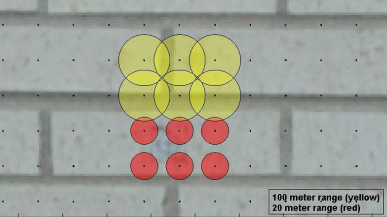
Yellow shows the diameter of the Optech’s beam at 100 meter range. The red shows the same beam at a 20 meter range

For distances greater than 500 meters and for expansive sites, airborne laser scanning (LiDAR) or traditional aerial photogrammetry are usually the preferred options. Survey Grade GPS may be an important component when surveying sites involving long-range distances as it allows you to relate extensive sites, dispersed features of interest, multiple technologies/setups and even periods of time with global coordinates.

Mid-range : For the 3D terrestrial scanners referenced on the GMV, ‘mid-range’ typically refers to distances between 1 – 140 meters. The effectiveness within this range depends on the scanner being used and, in some cases, on the reflectivity of the surface being captured. Low-altitude aerial photogrammetry and some terrestrial photogrammetery methods might also be used depending on the type of feature(s) being surveyed. For subsurface features, geophysics also becomes an option at this range as in most cases of CAST’s research, surveys explore the uppermost 5 meters of the earth’s surface. Again, GPS may play an important role in tying together a mid-range survey.

Close-range : For the 3D terrestrial scanners referenced on the GMV, ‘close-range’ typically refers to distances between 1 – 5 meters and it is often within 1 meter. At this range, Reflection Transformation Imaging (RTI) and Close-Range Photogrammetry (CRP) also become options. Deciding between scanning or photographic methods depends on whether 2D or 3D information is needed and on the time and resources at your disposal. Physical access to the object(s) or surface(s) also plays an important part in this decision.

[/wptabcontent]

[wptabtitle] SIZE OF FEATURES [/wptabtitle] [wptabcontent]

What is the size of the smallest feature of interest? The largest?

Answering this question in combination with an understanding of the range of distances involved, furthers your ability to identify which technologies are appropriate for your project.

Larger scaled features : If you are interested in surveying standing architectural structures/ ruins and/or interior spaces or rooms, there is a good chance that 3D scanning is a viable option. If you are interested in features within the structure, such as openings, archways, or larger-scaled details, this excludes long-range scanning as an option but it opens up photogrammetric options in addition to mid-range scanning.

Planimetric Features : In long-range scanning and low-altitude photogrammetry, capturing planimetric information for the structure(s) is possible but it is usually dependent on whether there is a covering/roof present and the height of the existing structure (i.e. whether the scan or photo is able to capture the geometry of the wall/ruin at the given distance). Multiple setups from elevated vantage points may help to capture the planimetric details from a distance. Capturing planimetric features is also possible with mid-range scanning, but it highly depends on the ability to tie together multiple scanner setups to form a legible layout of the structure(s). If you are interested in interior planimetric details, the presence of the roof is not typically relevant but access to setup the scanner from these interior spaces is required.

Finely scaled features : If you are interested in 3D information about more finely scaled details, such as shallow inscriptions or tool marks, close-range scanning typically becomes the preferred method of survey. However, if you are interested in less-precise 3D information or 2D information about these details or if you are interested in finely scaled details with very low/no physical relief, then RTI and CPR become reasonable options (note that RTI is restricted to 2D information with virtual 3D effects).

[/wptabcontent]

[wptabtitle] DATA RESOLUTION[/wptabtitle] [wptabcontent]

What data resolution do you need?

In general, when determining the proper resolution for your data, you should identify the smallest feature which you want to survey and the accuracy of the piece of equipment that you are using. Data resolution has different meanings as it is applied to different technologies.

In 3D scanning, resolution is defined as the average distance between the x, y, z coordinates in a point cloud. This is also called point spacing. In photographic methods, resolution is based on the dimensions of a pixel within the image.While it is tempting to simply say that you want the highest and most dense resolution that the technology will allow, it is important to realize that the higher the resolution the larger the file sizes and often, the longer the collection and processing times that are involved. For more detailed information on how resolution as it relates to heritage projects, see Archaeology Data Service / Digital Antiquity Guides to Good Practice

In Geophysics and GPS the accuracy of the data is often a more relevant consideration than the resolution of the data collected.

[/wptabcontent]

[wptabtitle] SITE/OBJECT CHARACTERISTICS [/wptabtitle] [wptabcontent]

Which technologies are appropriate for which characteristics?

While all sites and situations are different, there are some qualities that, if present, make certain survey methods more preferable than others. Deciding which technologies to use is largely based on characteristics of the site and/or object(s) and what type of information is needed. See the Survey Options for GMV Technologies table for a summary of the typical uses and abilities for the technologies at specific ranges given certain characteristics.

Common questions about the site and/or object(s) you wish to survey include:

I. Are there darkly colored, highly reflective (mirror-like), and/or translucent surfaces within the site that you want to capture?

II. What is the amount of relief and/or depth in the layer(s) of the surface being captured and what are the angles between these surface(s) and the equipment you are using?

III. Are there features or artifacts scattered across the site?

IV. Will subsurface features be included in your survey?

V. Is vegetation present on the site?

[/wptabcontent]

[wptabtitle] DARK, REFLECTIVE, TRANSLUCENT SURFACES [/wptabtitle] [wptabcontent]

Darkly colored, highly reflective (mirror-like) and translucent surfaces : All of these qualities affect the way in which 3D scanners interact with the surface being scanned, as does the smoothness or roughness of the surface.

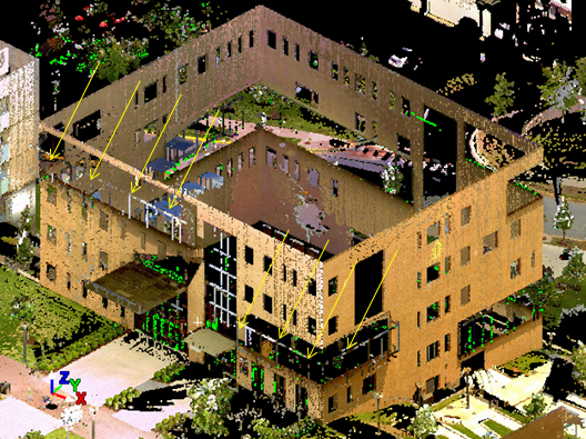
The yellow arrows indicate where the building’s black-colored windows should be. These darkly colored and translucent features were not captured with laser scanning.

The ability to collect surface data using a laser scanner (and the range at which it can be collected) is partially determined by the properties of the surface that is being recorded. In general terms, darkly colored surfaces absorb the laser beam while smooth, highly reflective (specular) surfaces reflect the beam at an angle equal to the incoming incidence angle (i.e. not back toward the scanner). Translucent surfaces partially transmit and diffuse laser beam. In all of these cases, the laser beam returning from surface can be extremely weak or nonexistent. If these surface qualities are very common within your site/feature(s) of interest, 3D scanning is probably not a good choice. However photogrammetric methods may be an option.

[/wptabcontent]

[wptabtitle] DEPTH & ANGLES OF THE SURFACE [/wptabtitle] [wptabcontent]

Angles of incidence, amount of relief/and or depth in the layer(s) within a surface :

Angles of Incidence: In terms of laser scanning, the angle of incidence is the difference between a perpendicular angle to the surface and the angle between the laser beam and the surface. Ideally, the laser should be perpendicular to the surface (i.e. the angle of incidence is 0°). The less perpendicular the laser and the surface are (i.e. the larger the angle of incidence) the more oblique and unreliable the data becomes. For example, scanning a building from the corner only would mean that the laser is not perpendicular to the walls of the building at any point, except the corner. The points on each wall would splay/widen as distance increases. So a flat wall would not have a regularized, gridded set of points to measure or analyze. While scanning a building’s corners is helpful in tying multiple scans together, if you are seeking accurate measurements on the walls, it is highly recommended to scan the walls from a perpendicular vantage point.

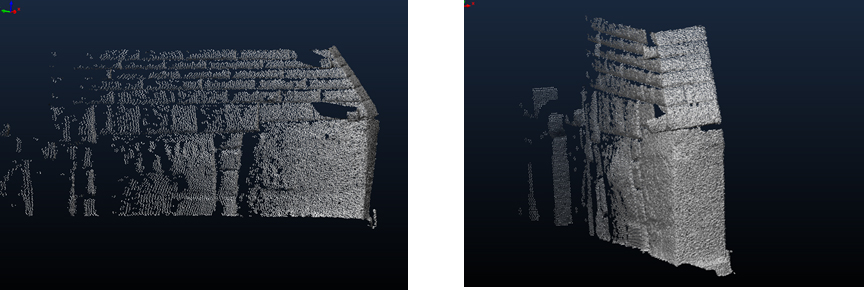
Left shows a stone wall scanned from a perpendicular angle; points are gridded evenly across the surface. Right shows the same wall scanned with a high angle of incidence. The density of the points changes as the distance and angle increases.

Relief & Depth within the Surface : The angle of incidence is especially important when considering surfaces that are highly detailed with multiple layers of relief. Multiple scanning positions are required to capture details reliably and depending on physical access and the size of the features, it may not be possible to capture all surfaces. Photogrammetric and RTI options may allow for greater flexibility and physical access to address some of these issues, although capturing all sides of highly complex, deeply recessed surfaces is problematic for any method.

[/wptabcontent]

[wptabtitle] SCATTERED OR SUBSURFACE FEATURES, VEGETATION [/wptabtitle] [wptabcontent]

Additional Qualities to Consider

In addition to the issues already discussed in detail in the previous slides, some other general questions that should be considered early in your planning process include:

Are there features or artifacts scattered across the site?

When features or artifacts are spread out across a site (i.e. single features or small areas of features are spread over significant distances) 3D scanning, CPR and RTI may be good options to record geometry and surface details. However, it will be difficult to relate the features to one another and to the greater site using these methods. In these cases, low-altitude photogrammetry and GPS are the preferred methods for tying together individual features or areas. If highly detailed geometric or surface information is needed, scans and/or photos can be tied together using GPS. If such highly detailed information is not needed, you can use GPS alone to record precise locations with specific semantic information (i.e. description of the ruin)and lower resolution geometric information (i.e. centimeter resolution outline of the perimeter of the ruin).

Will subsurface features be included in your survey?

If you are interested in features below the earth’s surface, utilizing geophysics becomes one of the primary methods used without actual excavation. At CAST, this type of survey usually focuses on the uppermost 5 meters of the earth’s subsurface. Oftentimes using geophysics in your survey can help you to identify and to prioritize areas for future research.

Is vegetation present on the site?

Vegetation can be problematic for a variety of reasons. To start, it can cover or obstruct features of interest so that scanning and photographic methods cannot properly record the surfaces themselves. A second problem caused by vegetation is its tendency to move. Changes in wind from one scan/photo to the next can cause serious problems when trying to align overlapping areas in which the human eye may be unable to identify the same point/area or in which the software may become confused over these multiple moving points.

Strategies for dealing with Vegetation : There are strategies for dealing with vegetation while collecting data, such as using the last laser return from a scanner vs. the first return (i.e. considering the last return to be the point at which the laser encounters the surface and considering the first return as the point at which the laser encounters the vegetation). Another strategy is to plan the survey during late fall/winter seasons when vegetation is at a minimum. There are also strategies for minimizing the impact of vegetation during processing, such as removing the tops of all trees before aligning scans.

[/wptabcontent]

[wptabtitle] PHYSICAL & TEMPORAL ACCESS [/wptabtitle] [wptabcontent]

Physical and Temporal Access to the Site

Temporal : It is difficult to estimate typical time frames for collecting data over a given area with a specific technology. Previous experience with the equipment and processes and the number of people on the site throughout the project greatly affect how long it will take to document a set of objects or sites. Other considerations include:

Time of day and year that you have access to the site (i.e. hours of daylight if daylight is needed).
Speeds of the specific equipment that you are using must be considered. With 3D scanning, there are significant differences in collection times depending on the scanner itself.
Transition time between setups often takes up a major portion of the overall time whether setting up for scans, photographs, or other methods of survey.
Weather, traffic and tourists are just a few of other interferences that might delay or change the course of data collection and should be considered specifically to your site.
Leaving a leeway/margin of time within the schedule is highly recommended (a minimum of roughly 1/3 the overall time is a good place to start).
Including processing time in field time is also highly recommended. Processing each day’s data as soon as possible, and if possible, before leaving the site can help you identify missing or corrupted data that cannot be replaced once you leave the site. Processing over a lunch break or when returning from the field each night is almost always worth the time.

Setting Priorities : Taking possible mishaps and delays into consideration, enter the site with a clear set of priorities.

What are the main objectives in the survey? What is essential to capture and what is secondary?
What is the total number of structures and/or features to be surveyed?
What resources (equipment, people) do you need to capture each survey objective? Arriving at the site prepared might make the difference between getting all of the data that you need or none of the data that you need.

Terrain : Many heritage sites are located ‘off the beaten track’. When planning the project, consider the total equipment weight, the number of people, and the overall ruggedness of where you will be hauling all of that weight. Have a clear understanding of the requirements for bringing equipment into different countries/regions in addition to knowing shipping and/or airline luggage regulations.

Power, Lighting : Consider power and lighting in your equipment calculation. Is there a power supply at the site? Do you need to haul batteries back and forth? Do you need to supply lighting for some areas/times?

[/wptabcontent]

[/wptabs]

Posted in Uncategorized

Assessing your 3D Model: Effective Resolution

[wptabs mode=”vertical”] [wptabtitle] Why effective resolution?[/wptabtitle] [wptabcontent]For many archaeologists and architects, the minimum size of the features which can be recognized in a 3D model is as important as the reported resolution of the instrument. Normally, the resolution reported for a laser scanner or a photogrammetric project is the point spacing (sometimes referred to as ground spacing distance in aerial photogrammetry). But clearly a point spacing of 5mm does not mean that features 5mm in width will be legible. So it is important that we understand at what resolution features of interest are recognizable, and at what resolution random and instrument noise begin to dominate the model.

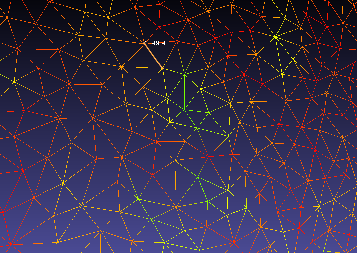
Mesh vertex spacing circa 1cm.

[/wptabcontent]

[wptabtitle] Cloud Compare[/wptabtitle] [wptabcontent]

The open source software Cloud Compare, developed by Daniel Girardeau-Montaut, can be used to perform this kind of assessment. The assessment method described here is based on the application of a series of perceptual metrics to 3D models. In this example we compare two 3D models of the same object, one derived from a C10 scanner and one from from a photogrammetric model developed using Agisoft Photoscan.[/wptabcontent]

[wptabtitle] Selecting Test Features[/wptabtitle] [wptabcontent]

Shallow but broad cuttings decorating stones are common features of interest in archaeology. The features here are on the centimetric scale across (in the xy-plane) and on the millimetric scale in depth (z-plane). In this example we assess the resolution at which a characteristic spiral and circles pattern, in this case from the ‘calendar stone’ at Knowth, Ireland is legible, as recorded by a C10 scanner at a nominal 0.5cm point spacing, and by a photogrammetric model built using Agisoft’s photoscan from 16 images.

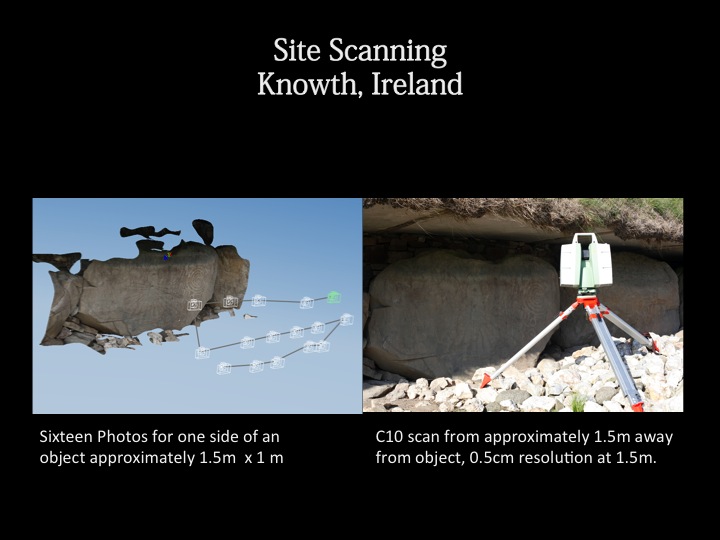[/wptabcontent]

[wptabtitle] Perceptual and Saliency Metrics[/wptabtitle] [wptabcontent]

Models from scanning data of photogrammetry can be both large and complex. Even as models grow in size and complexity, people studying them continue to mentally, subconsciously simplify the model by identifying and extracting the important features.

There are a number of measurements of saliency, or visual attractiveness, of a region of a mesh. These metrics generally incorporate both geometric factors and models of low-level human visual attention.

Local roughness mapped on a subsection of the calendar stone at Knowth.

Roughness is a good example of a relatively simple metric which is an important indicator for mesh saliency. Rough areas are often areas with detail, and areas of concentrated high roughness values are often important areas of the mesh in terms of the recognizability of the essential characteristic features. In the image above you can see roughness values mapped onto the decorative carving, with higher roughness values following the edges of carved areas.

[/wptabcontent]

[wptabtitle] Distribution of Roughness Values[/wptabtitle] [wptabcontent]The presence of roughness isn’t enough. The spatial distribution, or the spatial autocorrelation of the values, is also very important. Randomly distributed small areas with high roughness values usually indicate noise in the mesh. Concentrated, or spatially autocorrelated, areas of high and low roughness in a mesh can indicate a clean model with areas of greater detail.

High roughness values combined with low spatial autocorrelation of these values indicates noise in the model.

[/wptabcontent]

[wptabtitle] Picking Relevant Kernel Sizes[/wptabtitle] [wptabcontent]

To use the local roughness values and their distribution to understand the scale at which features are recognizable, we run the metric over our mesh at different, relevant, kernel sizes. In this example, the data in the C10 was recorded at a nominal resolution of 5mm. We run the metric with the kernel at 7mm, 5mm, and 3mm.

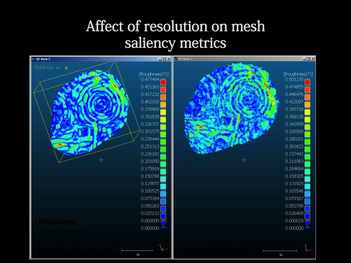
Local roughness value calculated at kernel size: 7mm.

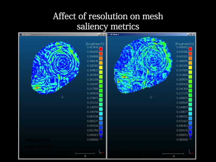
Local roughness value calculated at kernel size: 5mm.

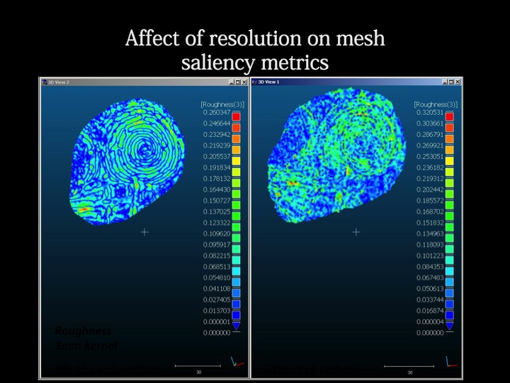
Local roughness value calculated at kernel size: 3mm.

Visually we can see that the distribution of roughness values becomes more random as we move past the effective resolution of the C10 data: 5mm. At 7mm the feature of interest -the characteristic spiral- is clearly visible. At 5mm it is still recognizable, but a little noisy. At 3mm, the picture is dominated by instrument noise.
[/wptabcontent]
[/wptabs]

Posted in Convergent Photogrammetry, Leica C10, Modeling, Photoscan | Tagged C10, data comparison, Photogrammetry, Photoscan Pro, Scanning

Basic Operation of the Epson 10000XL Flatbed Scanner with SilverFast Software Plugin for Photoshop

This document will guide you through using the Epson 10000XL Flatbed Scanner and SilverFast plugin to scan film for many applications including use in photogrammetry and archival storage.
Hint: You can click on any image to see a larger version.

[wptabs style=”wpui-alma” mode=”vertical”] [wptabtitle] GETTING STARTED [/wptabtitle]

[wptabcontent]

Transparency Unit – The EPSON 10000 XL scanner should have the transparency unit attached. If it is not attached, the user needs to turn off the power of the scanner, remove the regular cover, and attach the transparency unit. The transparency guide is not needed for scanning film.

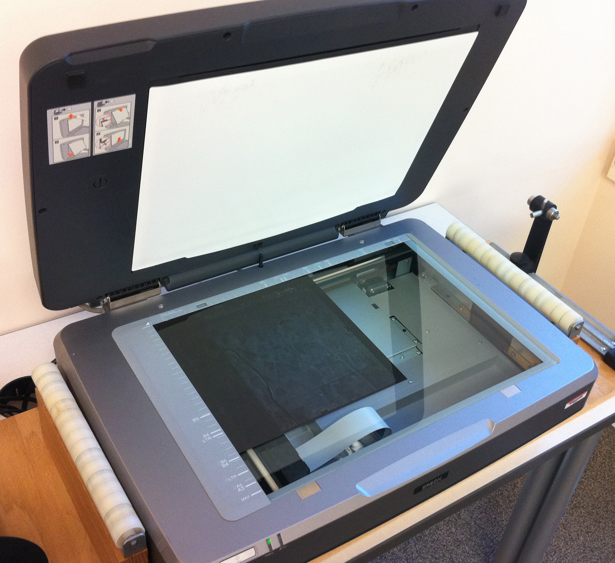
Epson 10000XL Flatbed Scanner

1 – Put on white gloves when handling film to avoid fingerprints rubbing onto film.

2 – Take film out of canister and find the glossy side, which will need to be face down for scanning.

3 – Unroll film to find flight direction markings, which are usually at the beginning of the roll. If there are none, then use your own judgment on flight direction so film data is correctly oriented.

4 – Put film on roller that allows film to feed through scanner with the glossy side down and with the data correctly oriented; switch spindles if necessary. This can be changed if the user later discovers that the film is incorrectly oriented.

5 – Push bars of rollers together to a distance with the film right between them and then tighten the knobs of the rollers.

[/wptabcontent]

[wptabtitle] PLACING FILM [/wptabtitle] [wptabcontent]

6 – Open Adobe Photoshop program and click on file, import, and select the Silverfast program.

7 – Roll the handle on the roller to feed film onto scanner. Film should be scanned at the top of the scanner. Rollers can be adjusted as necessary and scanner can be moved so the film is rolled across the top.

8 – When scanning portions of film that are not on the edge of the roll, attach the end of the film to the opening on the spindle of opposite roller.

9 – Once film is attached to spindle, use this roller to unroll and feed film through the scanner.

[/wptabcontent]

[wptabtitle] GENERAL SETTINGS [/wptabtitle] [wptabcontent]

10 – After Silverfast opens, click on Pre-Scan button at lower left corner for visualization of imagery. This provides an initial preview. Settings need to be changed as listed in the following step.

11 – Select the general tab and set the following settings:

1 – Scan mode-normal

2 – Original– reflective

3 – Pos/neg– positive

4 – Frame-set– save

[/wptabcontent]

[wptabtitle] SCAN QUALITY [/wptabtitle] [wptabcontent]

12 – Select the frame tab to control quality of scanning procedures and set
the following settings:

1 – Scan type – 16-8 bit grayscale

2 – Filter – GANE, to maximize dust and grain removal settings

3 – Setting – save

4 – Image type – standard

5 – Name – untitled, user can add a title when saving image

6 – Original– this setting displays the width and height of area being scanned and can be changed by typing in values or clicking and dragging on box in preview window.

7 – Scale – 100

8 – Q-factor – 2.5, maximizes quality of scan

9 – Screen – 480 lpi

10 – Scanning resolution is below screen and q-factor, but unlabeled, set to 1200 dpi

11 – Click pre-scan again for new preview of imagery. Re-size window to include only the area of film that contains data.

[/wptabcontent]

[wptabtitle] SCANNING [/wptabtitle] [wptabcontent]

13 – If desired, check additional options by clicking on options button at right corner to open extra options menu. These options do not need to be changed from default settings.

14 – If desired, check additional options located on top row of SilverFast menu, such as histogram and gradation curve adjustment – alter as the user sees fit. The auto-adjust tool is also located on this row and can improve scanned imagery if needed.

15 – Click on Scan button at bottom of tab to begin scanning imagery.

16 – Saving : Scanned imagery is loaded into Adobe Photoshop. The user needs to name the file and save it to a folder of your choice as a .tiff file.

[/wptabcontent]

[wptabtitle] FINISHING SCANS / GENERAL TIPS [/wptabtitle] [wptabcontent]

17 – Continue rolling film as needed to scan imagery and repeat scanning process.

18 – When finished scanning, use the roller on the original spindle to roll the film back.

TIPS

For clear scans : When scanning aerial photography, the user needs to either place sheets of paper behind the film or put the cover back over the transparency unit glass portion. It is also possible that this process could improve scanning results of other series as well.

Distortion : Each roll of film tightens as the user rolls the film through the scanner and attaches it to the roller on the opposite side. Occasionally, this results in the film becoming very tight and resists laying down flat on the scanner bed. When this happens, the portions of the scanned image on the edge of the scanner bed become distorted. Unrolling some of the film on the receiving roller relieves some of the tightness, but does not totally eliminate distortion from the image. The best way to eliminate the distortion is to select not to scan the area that is distorted during the pre-scan.

[/wptabcontent]

[/wptabs]

Posted in Setup Operations, Workflow, Workflow

Basic Operation of the Epson 10000XL Flatbed Scanner with EPSON Scan Utility Software

This document will guide you through using the Epson 10000XL Flatbed Scanner to scan photographs and other media for many applications including use in photogrammetry and archival storage.
Hint: You can click on any image to see a larger version.

[wptabs style=”wpui-alma” mode=”vertical”] [wptabtitle] GETTING STARTED [/wptabtitle]

[wptabcontent]
A current version of EPSON Scan Utility software can be freely downloaded from the Epson website and used to scan a variety of media, including transparent film and photographic prints.

Epson 10000XL Flatbed Scanner

To get started, make sure the scanner is connected to the computer and turn both the scanner and computer on. Log in to the computer and start the EPSON Scan software.

1. Mode – In the EPSON Scan dialog (Figure 1), change the “Mode” to “Professional Mode.”

2. Media – If scanning transparent film media, choose “Film” in the “Document Type” drop-down menu. If scanning paper, prints, or other reflective type media choose “Reflective.”

[/wptabcontent]

[wptabtitle] SETTINGS [/wptabtitle] [wptabcontent]

3. The “Document Source” should always be set to “Document Table.”

4. In the “Image Type” drop-down menu, choose the appropriate setting for the media you’re scanning.
-When scanning transparent film media we recommend using a 16-bit Grayscale (for B&W film) or 24-bit Color (for color natural or false color film).

Figure 1: Settings for scanning with EPSON Scan software

5. Choose a resolution that is appropriate for the media you’re scanning.

–   When scanning transparent film media we recommend using a minimum resolution of 1200 dpi
–   For high quality film, we recommend using 2400 or 3200 dpi in order to capture all of the available    detail contained within the film
–   When scanning print or paper media, a scanning resolution of 300-350 dpi should capture all of the    available detail contained within the print.

6. Un-check the “Thumbnail” check box. All other settings in the EPSON Scan dialog will depend on the media you’re scanning, or on your personal preference.

[/wptabcontent]

[wptabtitle] SCANNING [/wptabtitle] [wptabcontent]

Epson 10000XL Flatbed Scanner with Transparent Film on Scan Bed

Figure 2: Transparent Film on Scan Bed

7. Placement – Carefully place the media face down in the upper left corner of the scan bed (Figure 2). We recommend using clean gloves when handling transparent film or print media.

8. Click the “Preview” button at the bottom of the dialog and the scanner will begin scanning.

Figure 3: EPSON Scan software Preview

9. Once the preview scan is complete, the “Preview” dialog should appear (Figure 3). Use the Marquee tools to select the area of the media you would like to include in your scan. Be sure not to crop an image you plan on using for photogrammetry, and to include any visible fiducial marks.

10. Begin Scan – In the “EPSON Scan” dialog window, click “Scan” to start the scanning process.

[/wptabcontent]

[wptabtitle] SAVING YOUR FILE [/wptabtitle] [wptabcontent]

11. In the “File Save Settings” dialog, choose a location, format, and name for output file.

NOTE: For best practice (and especially projects considering archival), we recommend scanning to the TIFF (.tif) file format.

12. Time – Depending on the size of your media and the resolution you chose, the scanning process could take up to 1-2 hours.

[/wptabcontent]

[/wptabs]

Posted in Setup Operations, Workflow, Workflow | Tagged aerial photos, Epson, flatbed scanner, LPS, Photogrammetry, Photoscan, Photoscan Pro

Polyworks PIFEdit: Cleaning Point Cloud Data

This page will show you how to view and ‘clean’ the data in Polyworks PIFEdit.
Hint: You can click on any image to see a larger version.

[wptabs style=”wpui-alma” mode=”vertical”] [wptabtitle] POLYWORKS PIFEDIT [/wptabtitle]

[wptabcontent]

Introducing Polyworks PIFEdit:

PIFEdit is a data viewing and editing software available in the PolyWorks suite. It is used to clean scan data of unwanted data/points before importing the data into IMAlign.

* Note: You have to have a full license of Polyworks (w/dongle) to be able to edit and save data out of PIFEdit (otherwise it functions only as a viewer.

Basic Navigation:

Upon opening the PIF file in PIF Edit, view the scan using the appropriate mouse buttons:

Left Button: Rotates the scan

Middle Button: Translates the scan

Right Button: Zooms in and out on the scan

Get accustomed to the use and “feel” of these buttons because they are used in all of the PolyWorks modules.

[/wptabcontent]

[wptabtitle] VIEW DATA [/wptabtitle] [wptabcontent]

View the data from every angel to identify which data you want to keep and which data can be removed.

In this “un-cleaned” data the trees and people, in this case ROTC soldiers, are seen

In the image above, a group of ROTC soldiers were included in the scan. Since the focus of the scan is the building, the scan data of the soldiers, the trees, and the ground in front of the building will all be removed.

Notice how the trees and the soldiers (objects in the forefront) cause shadows or holes in the scan data of the structure (object in the rear). This can be remedied by simply acquiring another scan of the same area from another location if access and time permit another scan.

[/wptabcontent]

[wptabtitle] SELECT UNWANTED DATA [/wptabtitle] [wptabcontent]

To remove the unwanted scan data, press the space bar. This activates the Selection dialog box.

Hold down the Shift and Ctrl keys and use the middle mouse button to make your selection.

Shift: Enables Volumetric Selection – otherwise it is in Surface Selection mode which is only useful with polygon meshes

Ctrl: Enables Polygonal Selection – otherwise in Freeform Selection mode

[/wptabcontent]

[wptabtitle] CONFIRM SELECTION & DELETE DATA [/wptabtitle] [wptabcontent]

Because you have to perform a volumetric selection in PIFEdit (aka it selects everything in the selection window), it is always good to double check the integrity of your selection before you delete any data.

Once you have done so you can go ahead and delete the unwanted data points from the scan. Repeat this operation as many times as needed.

The red indicates data that has been selected. On the left we view the data from above, on the right we view the same selected data in a perspective view

When finished, go to File – Save As – save as name_cln.pf.

Note: Our naming convention is to tack a ‘cln’ onto the scan name or to put the cleaned data into a ‘clean’ subfolder. As a rule of thumb – never overwrite the original data.

[/wptabcontent]

[wptabtitle] CONTINUE TO… [/wptabtitle] [wptabcontent]

For further processing in the Polyworks Suite, continue on to Importing Data into IMAlign.

[wptabcontent]
[/wptabs]

Posted in Workflow | Tagged Data Processing, Data Viewing, ILRIS 3D, laser scanning, mid-range scanning, Optech, Polyworks

Optech ILRIS-3D Parser: Pre-Processing Scan Data

This page will show you how to process raw scan data from the Optech ILRIS in ILRIS Parser and how to view and ‘clean’ the data in Polyworks PIFEdit.
Hint: You can click on any image to see a larger version.

[wptabs style=”wpui-alma” mode=”vertical”] [wptabtitle] THE OPTECH PARSER[/wptabtitle]

[wptabcontent]

Introducing the Optech ILRIS-3D Parser:

The Parser program processes raw scanner data in a variety of output formats recognized by PolyWorks, GIS softwares, and other 3D modeling suites.

Using ILRIS Parser

Open the Parser program by double-clicking on the icon on your desktop. The Parser window displays as follows:

The Optech Parser window

[/wptabcontent]

[wptabtitle] ADD DATA[/wptabtitle] [wptabcontent]

Add your data

Add your .i3d file by clicking the “Add” button.

Browse to the scan file location and select the desired scan.

Adding data in Optech Parser

The .i3d file is added to the file window in the Parser. A photograph of the scanned area acquired by the laser scanner is also viewable in the Parser window.

[/wptabcontent]

[wptabtitle] OUTPUT FILES & GENERAL SETTINGS [/wptabtitle] [wptabcontent]

Next, specify your desired output file type. For more information on output file types and their respective settings, please refer to the ILRIS-3D Operation Manual (Section 9). The PIF file type is the default output file type and is a PolyWorks specific format for use in the Polyworks Suite. The PIF output options are discussed in the following slides.

Click on the “Settings” button.

General settings in Optech Parser

In the Output File Name textbox, specify the name and location for the output PIF file.

The Reduction option allows you to subsample your data (recommended subsampling: 1).

Filtering – You also have the option to “filter” your data by specifying a Range Gate and/or an Intensity gate.

The Range Gate option specifies a desired data range based on distance from the scanner (in meters)

The Intensity Gate option specifies a desired data range based on the intensity readings returned from the scanner. While it is good practice to range grade your data to remove outliers etc…, it is not required because the data can also edited in the PIFEdit software.

[/wptabcontent]

[wptabtitle] MORE GENERAL & ADVANCED SETTINGS [/wptabtitle] [wptabcontent]

General Settings:

It is recommended to leave the Generate Bitmap, Generate Log, and Output pf Intensity options checked.

Generate Bitmap creates a separate .bmp file of the scan photograph

Generate Log creates a report containing the scan statistics

Output pf Intensity adds the intensity values returned from the scanner to the PIF file.

General Details and Advanced Settings:

For more on these options and those available in the Advanced Settings tab, please refer to the ILRIS-3D Operation Manual (Section 9).

[/wptabcontent]

[wptabtitle] PARSE DATA [/wptabtitle] [wptabcontent]

When the desired options have been selected in the “Settings” menus, click “Ok,” and “Parse” the data. A progress report is displayed to show the steps and completion of the parsing process

The progress window shows as the data is being parsed

[/wptabcontent]

[wptabtitle] CONFIRM PARSING IS SUCCESSFUL[/wptabtitle] [wptabcontent]

Note that a green check appears beside the file name in the file window indicating that that the file has been parsed.

To view the resulting PIF file, click the “View output” button.

Confirm parsing was successful and view output file

[/wptabcontent]

[wptabtitle] VIEW PARSED DATA [/wptabtitle] [wptabcontent]

Once you click ‘View Output’ in ILRIS Parser, the PIF file is opened in the PIFEdit viewing window

The parsed file can now be viewed in PIFEdit

[/wptabcontent]

[wptabtitle] FILES CREATED IN PARSING [/wptabtitle] [wptabcontent]

Note that a PIF file (.pf), a report log (.txt) and a bitmap of the scan photo (.bmp) are created in the parsing process.

The files created in the parsing process

[/wptabcontent]

[wptabtitle] CONTINUE TO…[/wptabtitle]

[wptabcontent] Continue to Polyworks PIFEdit: Cleaning Point Cloud Data[/wptabcontent]
[/wptabs]

Posted in Checklist | Tagged Data Processing, ILRIS 3D, mid-range scanning, Optech, Polyworks

Optech ILRIS 3D: Set up and Basic Operation

These are basic set-up and operation instructions for operating the Optech ILRIS 3D with a laptop. See the Optech Manual that accompanies the scanner for more detailed information.

1. Set up the tripod as levelly as possible

2. Attach scanner to tripod, be sure to tighten screw securely

3. Turn on laptop and connect it to scanner using either the cable or wireless network. Depending on the desired configuration, please set up accordingly:

Ethernet/Wired Connection

– In Control Panel > Network Connections > Select Internet Protocol (TCP/IP)
– Use the following IP address: 192.9.202.1 and Subnet Mask: 255.255.255.0
– In I3dNet Software > Go to tools > Prefs > Communication > Enter 192.9.202.248
– Polyworks dongle

Wireless Connection

– In Internet Protocol (TCP/IP), enter the following IP address: 192.168.0.6 and Subnet Mask: 255.255.255.0
– In I3dNet Software > Enter IP address 192.168.0.5
– Note that to reset the IP address you can log onto the internet > In Control Panel > Network Connections > (TCP/IP) > Specify ‘Obtain IP Address Automatically’

4. Connect batteries to I-Bar in a T-shape. This is the only way that they will provide power to scanner

5. Connect batteries to scanner using battery cable

6. Start the I3DNet Program

7. Go to the Communication Menu > Click ‘Connect’

8. Click icon with red outline to place scanning area on screen and re-size red box to define the scan area

9. Click ‘Acquire’ button to obtain the distance to the object to be scanned

10. Set the parameters of the scan – First will return readings from the first object/surface that is encountered while Last will return readings from the last object/surface that is encountered. Use Last to scan ‘through’ objects such as trees, fences, etc.

11. Set point spacing of laser (resolution)

12. Press the apply button

13. Start scan and save the file in the desired location

14. Parse scan to check data quality

15. Continue to Optech ILRIS Parser: Pre-Processing Scan Data

Posted in Setup Operations, Workflows | Tagged Data Collection, ILRIS 3D, mid-range scanning, Optech

Optech ILRIS 3D: Equipment Checklist

Equipment Checklist – Confirm before leaving the lab!!

1. Tripod – DO NOT FORGET!!!
2. ILRIS 3D Scanner
3. Scanner Batteries – fully charged (4 total)
4. I-Bar/Battery Holder
5. Gray Battery Cable
6. Copy of Operation Manual
7. Operating Options :
- Laptop Option (Recommended) Requires:
- – Laptop with I3DNet, PIF Edit, and Parser software installed
- – External lithium battery – fully charged (2 options)
- – Modified Ethernet cable to connect to scanner OR two wireless cards (PCM 352 and LCM 352)
- – Polworks software (optional)
- – Polyworks dongle
- Palm Option Requires:
- – Handheld Palm Unit – fully charged with ILRIS 3D Palm software installed (different than I3DNet)
- – Serial data cable to connect to scanner
- – Flash card, flash card holder (to store data)
8. Optional Equipment:

– Extra scanner batteries

– Extra external laptop batteries

– Battery charger(s) for scanner batteries, laptop batteries, etc…

– AC/DC Car Charger

– Scan targets (optional)

– Digital Camera

– Metal rods (triangular)used for stabilizing tripod on hard surfaces

Posted in Checklist, Uncategorized

Pre-processing Digital Images for Close-Range Photogrammetry (CRP)

This page will show you how pre-process digital images for use in Close-Range Photogrammetry (CRP).
Hint: You can click on any image to see a larger version.

[wptabs style=”wpui-alma” mode=”vertical”] [wptabtitle] A BASIC INTRODUCTION [/wptabtitle]

[wptabcontent]

Why is pre-processing necessary?

For most close-range photogrammetry projects digital images will need to be captured in a RAW format, preserving the maximum pixel information which is important for archival purposes. Therefore it will likely be necessary to do some pre-processing in order to convert RAW images into a file format accepted by the photogrammetry software being used for the project.

If a color chart or gray card was using during image capture, it may also be useful to perform a white balance on the image set. There are a number of tools/software packages available for this purpose, but below we will describe a potential workflow using Adobe products for batch processing.

Overall steps of this workflow:

– Batch convert RAW to DNG (Adobe DNG Converter)
– Batch white balance (Camera Raw)
– Batch image adjustments (Camera Raw)
– Batch save to JPEG (or TIFF) format (Camera Raw)

[/wptabcontent]

[wptabtitle] BATCH CONVERT RAW DATA [/wptabtitle] [wptabcontent]

Batch RAW to DNG with Adobe Digital Negative (DNG) Converter Software

As an open extension of the TIFF/EP standard with support for EXIF, IPTC and XMP metadata, the Adobe DNG format is rapidly becoming accepted as a standards for storing raw image data (primarily from digital photography).

For more information about file formats for archival, see the Archaeological Data Service (ADS) Guides to Good Practice.

Steps to Batch Convert:

1. Download and install Adobe DNG Converter. As of the date this workflow was published, version 7.2 of Adobe DNG Converter is a free tool available for download on the Adobe website.

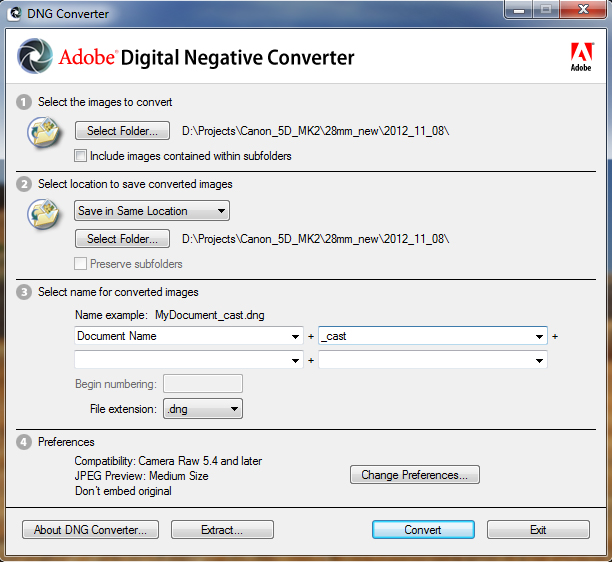
Adobe DNG Converter is a free tool available for download on the Adobe website.

2. This tool converts an entire folder (aka batch) of images at one time. Use the tool interface to select the appropriate input folder containing the RAW images.

3. If needed, use the interface to design a naming scheme to be used for the new file names.

4. Set preferences for compatibility (e.g. Camera Raw 5.4 and later) and JPEG Preview (e.g. medium size). As an option, you can embed the original RAW file inside the new DNG files. This will, or course, increase the file size of the new DNG file.

5. Click “Convert” to start the process. Wait for this to finish.

[/wptabcontent]

[wptabtitle] BATCH WHITE BALANCE – 1 [/wptabtitle] [wptabcontent]

Batch white balance, image processing, and exporting with Adobe – Part 1: Adobe Bridge

It is considered best practice to (correctly) use a quality color chart or gray card when capturing digital images for any CRP project. Performing a white balance for each image set (or each lighting condition) can dramatically enhance the appearance of a final product (i.e. ortho-mosaic). This particular workflow uses Adobe Bridge and the Adobe Camera Raw tool, but a similar process can be done in other (free) software as well.

Adobe Bridge – Open in Camera Raw

1. Open Adobe Bridge and navigate to the folder containing the digital images (DNG files).

2. Select the appropriate images (including images with color chart/gray card).

3. Use the “File” menu to select “Open in Camera Raw”

[/wptabcontent]

[wptabtitle] BATCH WHITE BALANCE – 2 [/wptabtitle] [wptabcontent]

Batch white balance, image processing, and exporting with Adobe – Part 2 : Camera Raw tool

4. Camera Raw will open and all of the selected images will appear on the left side of the window. Select the image with the color chart/gray card you would like to use for white balancing and other adjustments. Do all adjustments to this one image. We will apply the same changes to all images in the following slide ‘Batch Image Adjustment’.

Adobe Camera Raw – Image Processing Settings

5. By default, Camera Raw may attempt to apply a number of image processing settings that you should remove. This can be done using the interface on the right hand side of the screen. Check that all settings (with the exception of Temperature and Tint, which are set by the white balance tool in the next step) are set to zero. Be sure to check under each of the tabs.

6. Select the “Color Sampler Tool” found in tool bar at the top of the window and:

A. If using a color chart, add a color sample inside the black and white squares. After adding these you should see the RGB pixel values for each sample.

B. If using a gray card, add a color sample inside the gray portion of the card.

7. Select the “White Balance Tool” from the tool bar at the top of the window and click on the gray portion of the chart (or card) to apply a white balance. At the same time, notice how the RGB values of the color sample(s) change. The RGB values should not differ by more than five or six (e.g. the white sample could be R: 50, G: 50, B: 51). If they differ by too much there could be a problem with the white balance. Try clicking a slightly different spot in the gray portion of the chart.

8. If other adjustments need to be made (i.e. exposure, brightness, contrast) make them now.

[/wptabcontent]

[wptabtitle] BATCH IMAGE ADJUSTMENTS [/wptabtitle] [wptabcontent]

Applying adjustments to all

Once the white balance and adjustments have been made to this one image, we can apply the same to all the other images open in Camera Raw.

To do this, click “Select All” in the top left corner of the window – then click “Synchronize.” Wait for this to finish.

[/wptabcontent]

[wptabtitle] BATCH SAVE TO JPEG OR TIFF [/wptabtitle] [wptabcontent]

Saving

Once the Synchronization is complete, click the “Save Images” in the bottom left corner of the window (make sure all images are still selected). The “Save Options” dialog allows you to choose a folder for the images to be saved to, a naming scheme, a file extension and format, and a quality/compression. Choose the settings you prefer and click “Save.”

[/wptabcontent]

[wptabtitle] CONTINUE TO… [/wptabtitle] [wptabcontent]

Continue to PhotoScan – Basic Processing for Photogrammetry

[/wptabs]

Posted in Workflow, Workflow, Workflow, Workflow, Workflow | Tagged Adobe, Camera Raw, format dng, format jpeg, format jpg, format tif, format tiff, Photogrammetry, Photography Basics, PhotoModeler, PhotoModeler Scanner, Photoscan, Photoscan Pro, PhotoShop

Good Photos vs. Bad Photos for Close-range Photogrammetry

Close-range photogrammetry example from Ostia Antica, Italy. CAST, Uark

“Good” close-range photogrammetry example from Ostia Antica, Italy. Note that the object (the temple) is framed tightly, and that all objects (both near and far) are in sharp focus.

When it comes to close-range photogrammetry, the difference between “good” photos and “bad” photos can be the difference between getting useful 3D information and having complete failure. There are many different variables contributing to success or failure of a project, but to help avoid the most common mistakes a photographer can follow the general guidelines outlined below.

Basic photographic concepts that, when followed, generally produce acceptable digital images:

Camera/lens Properties:
-Use a mid to high resolution camera (at least 12-15MP)
-Use a fixed (non-zoom) lens
-Tape the focus ring (and set to manual focus)
-If using a zoom lens, tape the zoom ring and use one focal length for the entire project

Camera Placement:
-Use a tripod and stable tripod head
-Frame the subject tightly, making use of the entire sensor area
-Maintain 60-80% overlap between photos
-Ensure all important areas of the object are visible in at least three images
-Be aware of camera geometry required by software (baseline, convergent angles)

Camera Settings:
-Use aperture priority mode (set to between f/8 and f/16)
-Use a timer or wired/wireless shutter release to minimizes motion blur
-Use mirror lock-up, if available, to further minimizes motion blur

A list of common mistakes made while capturing digital images for a close-range photogrammetry project:

Camera/lens:

“Bad” close-range photogrammetry example. Note that the object (the temple) is not framed tightly, and that most objects are blurry and out of focus.

-Use of low resolution camera (8MP or less)
-Changing zoom (focal length) between images
-Use of loose/damaged lens
-Significant re-focusing due to varying distance from object

Camera placement:
-Handheld camera (no tripod)
-Insufficient overlap between images
-Inefficient use of sensor area (too far from subject)
-weak camera geometry (multiple images from one position, short baseline, overall poor network of image locations/orientations)

Camera settings:
-shallow depth of field (below f/8)
-manual shutter release (causes motion blur)

Posted in Checklist, Checklist, Checklist, Checklist, Setup Operation, Setup Operations, Setup Operations, Setup Operations | Tagged Canon 5D Mark II, Nikon D200, Nikon D70, Photogrammetry

ALS Processing: Assessing Data Quality

[wptabs mode=”vertical”] [wptabtitle] LAS files[/wptabtitle] [wptabcontent] ALS data is now usually delivered in the LAS format. The LAS format specification is maintained by the The American Society for Photogrammetry & Remote Sensing (ASPRS). The current version of the specification is 1.4. These files may be delievered as per-flightstrip or, more commonly from commercial vendors, as a collection of tiles.[/wptabcontent]

[wptabtitle] Metadata and Headers.[/wptabtitle] [wptabcontent]

Header information read by LASTools

Essential information about the data itself, organization and initial processing of a LAS file is contained in its header. Lidar processing software including LASTools and LP360 will allow you to access the LAS header information. It’s always a good idea to look at the headers to learn things like:

The software used to generate the file
The number of returns
The total number of points
Offsets and scale factors applied

Header information read by LP360

Many data providers will also supply a detailed project report including information on the project’s error budget, ground control networks, flight conditions, and other technical details. [/wptabcontent]

[wptabtitle] Checking the Point Density.[/wptabtitle] [wptabcontent]Knowing the real resolution of your lidar data is important. Checking that it matches your requested resolution is an essential part of quality control in an ALS project. This information will affect the parameters you select for classificaton and interpolation; It may also influence your expectations regarding the types of features you should be able to identify or accurately measure.

In LASTools you can use the ‘-cd’ or ‘-compute_density’ option in LASInfo to compute a good approximation of the point density for the file. Alternatively, you can use SAGA GIS, an open source GIS software package, to plot per grid cell density and visualize how the densities vary across your dataset.

Points per grid cell visualized in SAGA.

Histogram of points per grid cell, visualized in SAGA.

[/wptabcontent]

[wptabtitle]Sources of ALS Errors.[/wptabtitle] [wptabcontent]The total error for a lidar system is the sum of the errors from the laser rangefinder, the GPS and the IMU. These sources of error and the calculation of error budgets have been discussed extensively in the literature, including good summaries by Baltsavias (1999) and Habib et al. (2008). For ALS surveys conducted from fixed-wing aircraft platforms, these often total somewhere between 20 and 30cm.

The main sources of error are:

Platform navigational errors
GPS/IMU navigational errors
Laser sensor calibration errors (range measurement and scan angle)
Timing resolution
Boresight misalignment
Terrain and near-terrain object characteristics

Errors may be vertical (along the Z axis) or planimetric (shifts on the XY plane). The errors are obviously related, but they are usually quantified separately in accuracy reports. In commercial applications accuracy analyses usually focus on vertical accuracy, while planimetric accuracy (XY) is secondary.
[/wptabcontent]
[wptabtitle]Types of Errors.[/wptabtitle] [wptabcontent]Both horizontal and vertical errors may be described as random, systematic or terrain dependent. The main source of random error is position noise from the GPS/IMU system, which will produce noise in the final point cloud. These coordinate errors are independent of the flying height, scan angle and terrain.

Systematic errors include errors in range measurement, boresight misalignment, lever arm offset and mirror angle, and some errors from the GPS/IMU system (e.g. INS initialization and misalignment errors and multi-path returns). These errors will appear throughout the dataset. Terrain dependent errors derive from the interaction of the laser pulse with the ojects it strikes. In steeply sloping terrain or areas with off-terrain objects, and at higher scan angles, beam divergence may be increased and result in vertical errors due to horizontal positional shift.

Errors are most visually apparent in areas of strip overlap. A characteristic sawtooth pattern seen in hillshaded DTMs and clear misalignments of planar roof patches seen in the profile are typical of misalignment between adjacent strips.

Strip overlap errors seen in a hillshaded DTM.

Two scans of the same roofline in two overlapping strips are slightly offset, indicating a slight error. Points coloured by flightstrip.

[/wptabcontent]

[wptabtitle] Classification Errors.[/wptabtitle] [wptabcontent]Lidar data is typically gathered across large areas of the landscape, which may include woodland, urban and arable areas. One of the advantages of lidar over other remote sensing technologies is its ability to ‘see through’ the vegetation canopy, as some returns will pass through gaps in the canopy, reaching and returning from the ground- allowing the creation of a bare earth DEM. To accomplish this data must be classified (or filtered) to separate returns from terrain and off-terrain objects.

Points incorrectly classified as low vegetation (dark green) which should be terrain (orange).

There are a number of algorithms in use for classifying a point cloud. Regardless of the algorithm used, some errors will be committed. Two types of classification errors occur when performing a classification: the removal of points that should be retained (type 1) and the inclusion of points that should be removed (type 2). Overly aggressive algorithms or parameter settings have a tendency to remove small peaks and ridges in the terrain and to smooth or flatten the ground surface. Conversely, insufficiently aggressive parameters will induce the inclusion of clumps of low vegetation returns in the ground class, and can result in false ‘features’ [/wptabcontent] [/wptabs]

Posted in Airborne Laser Scanning | Tagged laser scanning, lidar, Scanning

Bayou Meto Lidar

ALS data from the Bayou Meto undergoing processing

CAST researchers and student assistants developed a hydro-enforced DTM (Digital Terrain Model) covering the Bayou Meto watershed, in collaboration with the NCRS and Arkansas Natural Resources Commission. The classification of the raw ALS data, interpolation to basic bare-earth terrain models, the creation of breaklines and streamlines for hydro-enforcement, and the refinement of final hydro-enforced models were carried out at CAST.

Data for this project was collected by Aeroquest in 2009 and 2010 for two areas within the Bayou Meto, at a nominal resolution of 10 pts/m2. The TIFFS and LP360 software packages were used to process the discrete return ALS data and to assist in breakline production.

For more information, see the main project webpage.

Posted in Airborne Laser Scanning Data | Tagged GIS/Remote Sensing, laser scanning, lidar

ALS Processing: Deliverables

[wptabs mode=”horizontal”] [wptabtitle] DTMs[/wptabtitle] [wptabcontent]ALS data can be used to create a number of products based on elevation data. The most common ALS product created is the bare earth DTM. The bare earth DTM provides the basis for analyses in hydrology, flood risk mapping, landslides, and numerous other fields.

Hydro-enforced DTMs include breaklines, importantly stream centerlines and edges, and breaklines delimiting standing water bodies such as ponds. While auto-extraction of breaklines is improving, the creation of hydro-enforcing features is still by and large a manual task.

Deliverables include hydro-DTMs.

[/wptabcontent]

[wptabtitle] DSMs[/wptabtitle] [wptabcontent]Digital Surface Models (DSMs) can include only returns from the terrain, buildings and specific classes of off-terrain objects like bridges, or can also incorporate returns from vegetation. DSMs are commonly used in urban environment analyses such as noise pollution modeling and inter-visibility analyses to assess the impact of new building.

DSMs are often used for modeling in urban areas.

[/wptabcontent]

[wptabtitle] CHM[/wptabtitle] [wptabcontent]Canopy height models, and per-stand or individual tree metrics are important ALS-based products for forestry applications. These models often include returns separated into low- mid- and high- vegetation classes, and are sometimes normalized based on local terrain heights to facilitate comparisons between different forest areas.

Canopy height model generated using SAGA GIS.

[/wptabcontent]

[wptabtitle] Contours[/wptabtitle] [wptabcontent]Contour maps at standard intervals, e.g. 1m, 5m, or 20m contours, can be generated from bare earth DTMs. Contour maps can be generated with or without breaklines.

Contours developed based on the terrain model.

[/wptabcontent] [/wptabs]

Posted in Airborne Laser Scanning Software | Tagged GIS/Remote Sensing, laser scanning, lidar, Scanning

ALS processing: Manual Re-classification

[wptabs mode=”vertical”] [wptabtitle] Initial Automatic Classification[/wptabtitle] [wptabcontent]In most ALS projects, in the first instance, the data is automatically classified. No automatic classification is perfect, and therefore visual assessment and the manual re-classification of some returns are important steps in the creation of a high quality hydro-enforced terrain model, and the development of other derivatives of ALS point clouds. The Bayou Meto terrain model developed at CAST was processed using TIFFS, a software program which implements a morphological filter. Other good low cost or open source software for automatic classification includes LASTools and MCC-Lidar.

Automatically classified Point Cloud seen in profile. Terrain points (class 2) are orange, and off-terrain points are grey.

[/wptabcontent]

[wptabtitle] Create DTMs and Hillshades[/wptabtitle] [wptabcontent]To facilitate visually identifying incorrectly classified returns, it’s useful to interpolate the automatically classified ground points into a DTM, and to create basic hillshades. Many classification errors will be readily apparent in the hillshaded models. The DTMs for the Bayou Meto project were created using LP360 for ArcGIS.

Bare earth DTM created before manual re-classification.

[/wptabcontent]

[wptabtitle] Linked Viewers[/wptabtitle] [wptabcontent]Viewing the point cloud simultaneously with the hillshaded terrain model, you can navigate quickly to ‘problem areas’ to re-classify any incorrect points in the ALS point cloud.

Linked viewers allow simultaneous viewing as a 3d point cloud, in profile, and at a shaded DTM.

[/wptabcontent]

[wptabtitle] Drawing Profiles[/wptabtitle] [wptabcontent]Draw a profile across an area of the terrain model where potential mis-classifications have been identified. Depending on how regular the terrain surface is, set the depth of the profile. Areas where the elevation of the terrain varies greatlygenerally require narrower profiles to clearly visualize the separation between the ground surface and low vegetation.

Drawing the profile on the DTM.

[/wptabcontent]

[wptabtitle] Editing classifications[/wptabtitle] [wptabcontent]When editing the classification of the points it’s best to set the point cloud coloring style to ‘by class’ rather than by elevation or by return, as it’s then easier to see which points should be re-classified. In LP360 you can change the classification of points by selecting them in the profile view using a ‘brush’ or ‘lasso’ tool and then typing the number of the class they should be and hitting enter. [/wptabcontent]

[wptabtitle] Typical problem areas[/wptabtitle] [wptabcontent]Work across the dataset systematically, until all problem areas have been improved. Note that areas with dense, low vegetation, large numbers of small buildings, and mixed steep slopes and vegetation are the most likely to contain mis-classified returns, and will require more effort. In the Bayou Meto dataset, the edges of streams proved typical problem areas, combining sloping terrain and low, dense vegetation.

Typical problem area circled in red, located under vegetation at the base of the slope.

[/wptabcontent]

[wptabtitle] Re-creating the terrain models[/wptabtitle] [wptabcontent]After re-classifying the ALS returns, it is necessary to re-create the terrain models and any other derivatives. These new models are the basis for further processing and analysis.

Hillshades and other derivatives are created from the cleaned point clouds.

[/wptabcontent] [/wptabs]

Posted in Airborne Laser Scanning Software | Tagged GIS/Remote Sensing, laser scanning, lidar

ALS Processing: Data Management

[wptabs mode=”vertical”] [wptabtitle] ALS data[/wptabtitle] [wptabcontent]ALS data is often collected in strips, with each strip representing an individual flightline. Typical ALS surveys have at least 20% overlap between adjacent flightlines and a few cross-strips where data is collected at an orientation perpendicular to that used for the main survey, improving accuracy.

A tie strip can be seen here overlapping with two flightlines.

[/wptabcontent]

[wptabtitle] Tile Schemes[/wptabtitle] [wptabcontent]Because ALS datasets are usually very large, they are often divided into regularly sized tiles. These tiling schemes can help with the speed of data loading, and allow users to load areas of the dataset selectively for processing or analysis.

Tiles represent .las file locations, one file is loaded. Note that the tiles are regular rectangles, and don't always exactly match the extents of the .las file.

[/wptabcontent]

[wptabtitle] LP360 tiling tools[/wptabtitle] [wptabcontent]LP360, like most ALS software, provides tools to perform the tiling task. Typical tile sizes include 0.5×0.5km or 1x1km tiles. The naming convention for the tiles should follow a sensible progression, for example reflecting official map grid designations for the area, or following an east to west progressive sequence across the survey area.

The LP360 .las subsetting tool

[/wptabcontent]

[wptabtitle] Creating Footprints[/wptabtitle] [wptabcontent]A vector file containing the footprints for each tile, designating the area covered and linking to the .las file or derived terrain models, are a common way of efficiently representing the ALS dataset in a GIS environment. Using LP360, individual files or groups of files can be loaded by selecting their footprints.

Las file footprints are outlined in dark blue; a selected footprint is highlighted.

[/wptabcontent]

[wptabtitle] Metadata[/wptabtitle] [wptabcontent]Metadata for ALS is typically generated for the entire survey, rather than per tile. This project level metadata is usually stored in a long form report. That said, some metadata will be stored in the .las header for each tile. Attributes including the total number of points in the file, whether or not it has been classified, and the software used to process the data are typical items found in the header. Further, non-standard, metadata can be stored as a series of attributes in the vector footprint for each .las tile.

Project level metadata provided by the vendor, Aeroquest, provides important information about the survey.

[/wptabcontent]

[wptabtitle] laz compression[/wptabtitle] [wptabcontent]The ASPRS standard .las format is commonly used for storing ALS data. The compressed .laz format is also useful, particularly for the datasets which are being archived. Data can be converted from .las to .laz (and back) using LASzip.
[/wptabcontent]
[/wptabs]

Posted in Airborne Laser Scanning Software | Tagged GIS/Remote Sensing, lidar, Scanning

ALS and Archaeology

[wptabs mode=”vertical”] [wptabtitle] ALS and Archaeology.[/wptabtitle] [wptabcontent]

Hillshaded lidar terrain model revealing (undated) remains of field systems now located within the Chailluz Forest, France. ALS Data credit: Region de Franche-Comté / MSHE Ledoux

Airborne Laser Scanning (ALS), or lidar, has been described as one of the most important innovations in data collection and interpretation for archaeology in recent years (Bewley et al. 2005). Certainly, ALS has become an important part of the archaeologists toolkit. First, and perhaps foremost, it has been employed in mapping and prospection surveys in woodland, scrub and open ground. Critically, it may provide the only means of survey -and consequently the collection of archaeological information- in difficult to access areas. Beyond prospection, ALS is now used in research and cultural heritage managements tasks ranging from assessments of the impact of hydrology on site locations, to the calculation of inter-visibility of a network of sites, to the analysis of landforms to create inputs for predictive modeling. The popularity of ALS for studying forested areas, floodplains and rural areas in general has renewed interest in the topic of topographic survey, and further spurred integration with digital technologies and applications. The growing use of ALS in archaeology has raised a number of issues, briefly outlined here.[/wptabcontent]
[wptabtitle] Basic Processing and Classification. [/wptabtitle] [wptabcontent]

Points incorrectly classified as low vegetation (dark green) which should be terrain (orange).

Archaeological applications demand high quality processing and classification of the ALS data. Because many buried or surface archaeological features are both small scale (in xy) and low relief (in elevation) and are often in woodlands or other heavily vegetated areas, good alignment within the point cloud is necessary to minimize noise, and a good classification is necessary to distinguish between low vegetation and low relief terrain features which may represent archaeological remains.[/wptabcontent]

[wptabtitle]Visualization.[/wptabtitle] [wptabcontent]Processing and visualization clearly affect interpretations. There are many possibilities to generate new models and visualizations, and a concurrent possibility of continually tweaking parameters in the hope of ‘improving’ the model. Archaeologists undertaking a project using visualizations should pose two questions. First, how much information can be retrieved, and with how much effort? Crutchley (Cowley and Opitz 2013) observes that if one model gives 90% of the nominal ‘total’ information, then the decision not to chase the other 10% may be a practical one. This pragmatic approach avoids the dangers of loosing sight of survey objectives in an endless round of data processing and manipulation. However, assessing the cost/benefit and deciding where to stop data manipulation, because a certain approach gives enough information for the task at hand, is not always obvious.

Sky View Factor visualization of karstic terrain. Schematics image credit: Zaksek et al., 2011

Popular 2D visualizations of bare earth DTMs in archaeology include:

-Classic Hillshades
-Multi-Directional Hillshades
-Slope Maps
-Sky View Factor
-PCA of multiple Hillshades

Simultaneous viewing of the point cloud, in profile or as a 3D model, alongside the shaded terrain model is common practice. The combined information from multiple views of the same data helps interpreters to understand if a small bump is likely to be a potentially archaeological mound, or built up soil around the base of a particularly large tree, not fully removed by the filtering process.
[/wptabcontent]

[wptabtitle] Metadata about Visualizations. [/wptabtitle] [wptabcontent]Providing detailed information on how a model and visualization was created is essential for others to understand and evaluate the end product and interpretation. Kokalj et al. (in Cowley and Opitz, 2013) recommend metadata about processing and visualizations as follows:

-data scanning: scanner type, scanning density, density of a combined dataset, scanning date;
-data processing: method(s) used, parameter settings, description of the processing goal (e.g. producing a terrain model, removing just the vegetation), elevation model resolution;
-visualization: method(s) used, parameter settings (e.g. hillshading (Sun elevation and azimuth), LRM (method, distance), SVF (distance, directions);
-interpretation process: reliability of the results (qualitative if quantitative evaluation is not possible, e.g. low to high, description of each class is recommended).

[/wptabcontent]

[wptabtitle] Analyses Using lidar DTMs. [/wptabtitle] [wptabcontent]The detailed terrain models produced from ALS data are used in archaeological research and cultural resource management as inputs for a number of analyses. These include:

-Visibility Studies
-Predictive Modeling
-Least Cost Path and Cost Surface Modeling
-Erosion Assessments

Viewsheds calculated based on the lidar DTM of the Boyne Valley, as observed from Newgrange. Image credit: Opitz and Davis, AARG 2012

[/wptabcontent]

[wptabtitle] External Resources.[/wptabtitle] [wptabcontent]

The ArchaeoLandscapes Project is an EU based project promoting the use of remote sensing and surveying technologies in archaeology. Their website is an excellent resource for both general information and case studies about the use of ALS in archaeology.

The English Heritage Guide to Airborne Laser Scanning provides good information on the use of ALS in the context of a national cultural heritage management organization.[/wptabcontent] [/wptabs]

Posted in Airborne Laser Scanning | Tagged Archaeology/Historic Recordation, lidar

Gabii Photogrammetry

The Gabii Project is an international archaeological project, directed by Nicola Terrenato of the University of Michigan. The Gabii Project began in 2007, seeking to study the ancient Latin city of Gabii through excavation and survey. Gabii, located in central Italy, was a neighbor of and rival to Rome, and flourished during in the first millennium BC.

The excavations at Gabii are uncovering extensive and complex remains within the city’s urban core. Convergent photogrammetry is essential to the project’s recording strategy. At Gabii, this technique is used to document features with complex geometries or large numbers of inclusions, including walls, pavements, rubble collapse, and architectural elements. These types of features can be quite time-consuming to document thoroughly by hand or using conventional surveying in the field. The 3D models collected in the field are georeferenced. They are subsequently simplified for incorporation into the project’s GIS, and compiled into models for distribution online using Unity3D.

You can see a sample model in the Unity3D interface here. You will need to download and install the free Unity webplayer to view the model.

View Gabii Project in a larger map

Posted in Convergent Photogrammetry, Photogrammetry Data | Tagged Archaeology/Historic Recordation, Photogrammetry, Photoscan Pro

Knowth Photogrammetry

Detail from the model of the K11 kerbstone, showing decorative carving on the rock surface.

The archaeological complex at Knowth, located in the Brú na Bóinne World Heritage Site, consists of a central mound surrounded by 18 smaller, satellite mounds. These monuments incorporate a large collection of megalithic art, primarily in the form of decorated stones lining the mounds’ internal passages and surrounding their external bases. The megalithic art found at this site constitutes an important collection, as the Knowth site contains a third of the of megalithic art in all Western Europe. The kerbstones surrounding the main mound at Knowth, while protected in winter, sit in the open air for part of the year, and are consequently exposed to weather and subject to erosion. The Researchers at CAST, in collaboration with UCD Archaeologists and Meath County Council, documented the 127 kerbstones surrounding the central mound at Knowth over the course of two days using close range convergent photogrammetry. This pilot project aims to demonstrate the validity of photogrammetry as the basis for monitoring the state of the kerbstones and to add to the public presentation of the site, incorporating the models into broader three dimensional recording and documentation efforts currently being carried out at Knowth and in the Brú na Bóinne, including campaigns of terrestrial laserscanning and aerial lidar survey.

The k15 kerbstone is available here as a sample dataset. You can download the 3D pdf (low res) or the DAE file (high res).

Photogrammetry data from this project was processed using PhotoScan Pro.

Photoscan Pro processing of the model for the K15 kerbstone.

View Knowth TLS and Photogrammetry in a larger map

Posted in Convergent Photogrammetry, Photogrammetry Data | Tagged Archaeology/Historic Recordation, Photogrammetry, Scanning

Microsoft Kinect – Setting Up the Development Environment

[wptabs mode=”vertical”]
[wptabtitle] Using Eclipse IDE[/wptabtitle] [wptabcontent]Since there is a plethora of existing tutorials guiding how to set up various development environments in C++, I will show you how to set up the 32-bit OpenNI JAR (OpenNI Java wrapper) in Eclipse IDE and to initialize a production node to begin accessing Kinect data via the Java programming language.
To continue we will be working with the open-source and fantastic piece of software known as Eclipse that you can find here: www.eclipse.org. You will want to download the IDE for Java programmers located on their “downloads” page(about 149 mb). Take note of the many other software solutions that they offer and the vast amount of resources on the site.

NOTE: Even though we are downloading the “Java” Eclipse IDE you can easily add plugins to use this same piece of software with Python, C/C++, and many other applications.

Additionally, we are assuming that you have already gone through the OpenNI installation located here.

You also need to have the Java JDK installed (www.oracle.com).

Finally, to gain access to one of the best open-source computer vision libraries available, you will need to download and install OpenCV(http://opencv.org/) and the JavaCV(http://code.google.com/p/javacv/). The installation instructions located on each of these sites are excellent.
[/wptabcontent]

[wptabtitle] Setting Up Eclipse with OpenNI: Before You Start[/wptabtitle] [wptabcontent]

Important Note: As you may already be aware, these tutorials are focused on the Beginner Level user, not only to using the Kinect but also to programming. Before going any further I should also remind you that if jumping “head first” into the new domain of programming isn’t something for which you have the interest or the time, there are many things you can accomplish with the “ready to use software” solutions located here.

Also, before starting, make sure that you are using the same platform (32 –bit to 32-bit/64 to 64) on the Eclipse IDE, Java JDK, and OpenNI installation.

[/wptabcontent]

[wptabtitle] Eclipse with OpenNI: Starting a New Java Project [/wptabtitle] [wptabcontent]

Starting a New Java Project …..
Once you have downloaded Eclipse, installed the java JDK and the OpenNI/Primesense, you will need to start a new Java Project. Following the wizard is the easiest way to do this.

Check the box that says “public static void main(String[] args)” so that Eclipse will add a few lines of code for us.

NOTE: For this tutorial I have kept the names fairly vague – be sure to use names that you will remember and understand. Remember that if you use a different naming convention than shown here, you will need to make corrections in the sample code to fit to your specifications.

[/wptabcontent]

[wptabtitle] Eclipse with OpenNI: Adding the OpenNI Libraries Part 1[/wptabtitle] [wptabcontent]Adding the OpenNI libraries…

Next we will need to add the OpenNI libraries to the project. This is a pretty straight forward process in Java and Eclipse, simply being a matter of adding the pre-compiled JAR file from the “bin” folder of your OpenNI installation directory.

NOTE: If you plan on using User Tracking or another Primesense middleware capability you will need to add the JAR in the Primesense directory

To do so right-click on the project we just created:

And select the “Properties” menu item.
Then we will want to select the “Java Build Path” and “Add External Jar’s” button.

Repeat the same steps as above for the JavaCV JAR’s that you previously installed somewhere on your machine.

[/wptabcontent]

[wptabtitle] Eclipse with OpenNI: Adding the OpenNI Libraries Part 2[/wptabtitle] [wptabcontent]

Navigate to the “bin” folders of the install directories for OpenNI and Primesense.
On my Windows 7 64-bit machine with the 32-bit install it is located here:

Note: There are TWO OpenNI “JAR” files – one in the bin folder of the OpenNI install directory as well as one in the Primesense directory. I haven’t noticed any difference in using one over the other; as long as your environment paths in Windows are set up to locate the needed files, they should both work.

After this, you should see these files in the “Referenced Libraries” directory on the “Package Explorer” tool bar in Eclipse.

[/wptabcontent]

[wptabtitle] Eclipse with OpenNI: Projects [/wptabtitle] [wptabcontent]

We should now be able to access the Kinect via Java and Eclipse.

In the following projects we will introduce and attempt to explain the necessary steps for initializing the Kinect via OpenNI and for getting basic access to its data feeds in Java.

Each project goes through setting up the Kinect in OpenNI and includes comments to explain line-by-line what is going on.
[/wptabcontent]

[wptabtitle] For information on Visual Studio 2010 & Microsoft C# SDK….[/wptabtitle] [wptabcontent]Using the Microsoft SDK provides a lot of advantages and ease of access, but it is also only applicable to the “Kinect for Windows” hardware and not the Xbox Kinect (as of v1.5).

There are a lot of existing tutorials on the web about setting up your development environment with plenty of sample projects. Below is a list of links to a few of them in no particular order as to avoid reinventing the wheel.

[/wptabcontent]

[/wptabs]

Posted in Microsoft Kinect, Uncategorized | Tagged close range scanning, computer vision, java, Kinect, laser scanning, Modeling, opensource, Photogrammetry, programming, Scanning, Workflow

Microsoft Kinect – Sample RGB Project

[wptabs mode=”vertical”]
[wptabtitle] Overview[/wptabtitle] [wptabcontent]As previously mentioned, the OpenNI API is written in C++ but once you follow the installation procedures covered, here, you will have some pre-compiled wrappers that will give you access to use OpenNI in a few other languages if you need.

Since there is a plethora of existing tutorials regarding setting up various development environments in C++ and corresponding example projects, this article will show you how to setup the 32-bit OpenNI JAR (OpenNI Java wrapper) in Eclipse IDE. We will then initialize an OpenNI production node to begin accessing Kinect data and to get the RGB stream into OpenCv, which is a popular computer vision library.

Before going on to the following project, make sure that you have all of the dependent libraries installed on your machine. For the instructions on getting the 3rd party libraries and for setting up the development environment check out this post.

Also, I want to clarify that this code is merely one solution that I managed to successfully execute. This said, it may have bugs and/or mayb be done more successfully or more easily using a different solution. If you have any suggestions or find errors, please don’t hesitate to contact us and I will change the post immediately. These posts follow and continue to follow exploration and collaboration.

[/wptabcontent]

[wptabtitle] Using the Kinect’s RGB feed[/wptabtitle] [wptabcontent]

[/wptabcontent]

In this project we will:

Make a simple program to capture the RGB feed from the Kinect in Java

Get the data into an OpenCV image data structure

Display the data on the screen

A high-level overview of the steps we need to take are as follows:

Create a new ‘context’ for the Kinect to be started

Create and start a ‘generator’ which acts as the mechanism for delivering both data and metadata about its corresponding feed

Translate the raw Kinect data into a Java data structure to use in native Java libraries

Capture a “frame” and display it on screen

The next tab is the commented code for you to use as you wish.

NOTE: For extremely in-depth and excellent instruction on using JavaCV, the Kinect, along with various other related projects I extremely the book(s) by Andrew Davison from the Imperial College London. A list of his works can be found here http://www.doc.ic.ac.uk/~ajd/publications.html and here http://fivedots.coe.psu.ac.th/~ad/.

[wptabtitle] Sample RGB Project – Part 1[/wptabtitle] [wptabcontent]

[/wptabcontent]

First, let’s import the required libraries:

import org.OpenNI.*;

import com.googlecode.javacv.*;
import static com.googlecode.javacv.cpp.opencv_imgproc.*;
import com.googlecode.javacv.cpp.opencv_core.IplImage;

Then eclipse nicely fills out our class information.

public class sampleRGB {

We define some global variables

static int imWidth, imHeight;
static ImageGenerator imageGen; static Context contex

Eclipse will also fill out our “main” statement for use by checking the box on the project set up. One addition we will need to make is to surround the following code block with a statement for any exceptions that may be thrown when starting the data feed from the Kinect. Here we are starting a new “context” for the Kinect

public static void main(String[] args) throws GeneralException {
Create a “context”

context = new Context();

[wptabtitle] Sample RGB Project – Part 2[/wptabtitle] [wptabcontent]

[/wptabcontent]

We are manually adding the license information from Primesense. You can also directly reference the xml documents located in the install directory of both the OpenNI and Primesense.

License license = new License("PrimeSense", "0KOIk2JeIBYClPWVnMoRKn5cdY4="); context.addLicense(license);

Create a “generator” which is the machine that will pump out RGB data

imageGen = ImageGenerator.create(context);

We need to define the resolution of the data coming from the image generator. OpenNI calls this mapmode (imageMaps, depthMaps, etc.). We will use the standard resolution.

First initialize it to null.

MapOutputMode mapMode = null; mapMode = new MapOutputMode(640, 480, 30); imageGen.setMapOutputMode(mapMode);

We also need to pick the pixel format to display from the Image Generator. We will use the Red-Green-Blue 8-bit 3 channel or “RGB24”

imageGen.setPixelFormat(PixelFormat.RGB24);

[wptabtitle] Sample RGB Project – Part 3[/wptabtitle] [wptabcontent]

[/wptabcontent]

OpenNI also allows us to easily mirror the image so movement in 3d space is reflected in the image plane

context.setGlobalMirror(true);

Create an Iplimage(opencv image) with the same size and format as the feed from the kinect.

IplImage rgbImage = IplImage.create(imWidth,imHeight, 8, 3);

Next we will use the easy route and utilize JFrame/Javacv optimized canvas to show the image

CanvasFrame canvas = new CanvasFrame("RGB Demo");

Now we will create a never-ending loop to update the data and frames being displayed on the screen. Going line by line we will, update the context every time the image generator gets new data.
Set the opencv image data to the byte buffer created from the imageGen.

NOTE: For some reason the channels coming from the Kinect to the opencv image are ordered differently so we will simply use the opencv convert color to set the “BGR” to “RGB”. We tell the canvas frame that we created to show image.

[wptabtitle] Sample RGB Project – Part 4[/wptabtitle] [wptabcontent]

[/wptabcontent]

Finally, we need to also release the Kinect context or we will get an error the next time we try to start a node because the needed files will be locked

while (true){ context.waitOneUpdateAll(imageGen); rgbImage.imageData(imageGen.createDataByteBuffer()); cvCvtColor(rgbImage, rgbImage, CV_BGR2RGB); canvas.showImage(rgbImage);

canvas.setDefaultCloseOperation(CanvasFrame.EXIT_ON_CLOSE); }

**Note that you can add an argument to the canvas frame to reverse the channels of the image

[/wptabs]

Posted in Microsoft Kinect, Uncategorized | Tagged computer vision, java, Kinect, laser scanning, Modeling, opensource, Photogrammetry, programming, Scanning

Working with the Vue interface with Python

[wptabs style=”wpui-alma” mode=”horizontal”] [wptabtitle]Passing arguments[/wptabtitle]
[wptabcontent]
The snippet below launches Vue from a Python script and passes in two arguments to Vue, ARG1 and ARG2:

import subprocess
command = [r"C:\Program Files\e-on software\Vue 10.5 Infinite\Application\Vue 10.5 Infinite", "-p'D:\\Temp\\bat-test.py' ARG1 ARG2"]
result = subprocess.Popen(command)

[/wptabcontent] [/wptabs]

Posted in Modeling, Vue Infinite | Tagged 3D, gis, python, scripting, VUE

Working with objects in Vue with Python

[wptabs style=”wpui-alma” mode=”horizontal”]
[wptabtitle]Get the size of an object[/wptabtitle]
[wptabcontent]Getting the actual size of an object in Vue programmatically isn’t as easy as you’d think. You essentially have to get the BoundingBox of the object and work with that. So here we have a wind turbine object, and we have selected the pole and need to know (programmatically) how tall this pole really is.

If you look at that z-value in the size properties, you see that it’s 76.045m tall. To get that height programmatically (result on line 21):

#
#
>>> col = GetSelectedObjectByIndex(0)
>>> col
>>> scale = col.GetScale()
>>> print scale
(1.0, 1.0, 1.0)
>>> bb = col.GetBoundingBox()
>>> print bb
<VuePython.VUEBoundingBox; proxy of <Swig Object of type 'VUEBoundingBox *' at 0x0000000017884360> >
>>> print bb.GetMax()
(4024.3647753980426, -9026.798040135702, 216.7754350035159)
>>> print bb.GetMin()
(4019.764775016573, -9031.39804242452, 140.730600866553)
>>> 

# Do the math

>>> z_size = bb.GetMax()[2] - bb.GetMin()[2]
>>> print z_size
76.044834137
>>> 

# Make a dict out of em

>>> d = {}
>>> d['Min'] = bb.GetMin()
>>> d['Max'] = bb.GetMax()
>>> print d
{'Max': (4024.3647753980426, -9026.798040135702, 216.7754350035159), 'Min': (4019.764775016573, -9031.39804242452, 140.730600866553)}
>>>
>>> print d['Max'][2]
216.775435004
>>>
#
#

[/wptabcontent]
[wptabtitle] Multiple cameras[/wptabtitle]
[wptabcontent]
Turns out there is no Python method in the Vue API for creating a camera. In order to create cameras, you can duplicate the Main camera and then call your custom cameras by index, where the index is the ID number of the camera.

#
#
# Dict of KOPs and attributes
# {KOP ID: (northing, easting, cam z position, FoV,    
#           camera yaw, camera pitch,  sun pitch, sun yaw)}
d = {5: ('15980.6638981', '6893.65640636', '3.7', 'Center', 
         '344.064664362', '93', '116.821439116', '120.778962736'), 
     6: ('8647.62696908', '27858.4046614', '3.7', 'Center', 
         '283.801779018', '93', '116.693562607', '120.534961058')}

# Create new cameras by duplicating Main camera for each KOP
for k in d.iterkeys():
    sc = SelectByName("Main camera")
    camera = GetSelectedObjectByIndex(0)
    Duplicate()
    DeselectAll()

# Set start position to 2, as its zero based indexing and Main camera is 0, 
#  Top camera is 1, so our first custom camera will be 2
cam_start_pos = 2

# For each pair in kop dict, map it to a new dict, where key is camera 
#  index and value is kop dict kv pair
#  {2:{'5': ('15980.6638981', '6893.65640636', '3.7', 'Center', 
#            '344.064664362', '93', '116.821439116', '120.778962736')},
#   3:{'6': ('8647.62696908', '27858.4046614', '3.7', 'Center', 
#            '283.801779018', '93', '116.693562607', '120.534961058')}}
i = 2
cams_kops = {}
for k, v in d.iteritems():
    cams_kops[i] = dict([(k, v)])
    i+=1
  
# Get the kop id (its a dict key) for a given camera id
cams_kops[2].keys() # 5

# Setup the camera for each KOP
select_camera = SelectByName("Main camera")
for k, v in cams_kops.iteritems():
    if SwitchCamera(k):  # k is camera id
        #kop_id = cams_kops[k].keys()[0]
        kop_attributes = cams_kops[k].values()[0]        
        camera = GetSelectedObjectByIndex(0)
        camera.SetPosition(float(kop_attributes[1]), 
                           float(kop_attributes[0]), 
                           float(kop_attributes[2]))
        Refresh()
        camera.SetRotationAngles(float(kop_attributes[5]), 
                                 0, float(kop_attributes[4]), true)
        Refresh()           
    else:
        # raise exception
        print "No"
        
    i+=1
    
# Create KOP/camera dictionary {KOP:camera id, ..} to associate each
#  KOP with its camera
kop_camera_ids = {}
for camera_id, kop_id in cams_kops.items():
    kop_camera_ids[kop_id.keys()[0]] = camera_id
    
print kop_camera_ids

SwitchCamera(0) # Activates "Main camera" again

# Now to switch the camera to a known KOP ID's camera, just do:
SwitchCamera(kop_camera_ids[6]) # call camera by the KOP ID
#
#

This results in two new cameras, Main camera0 and Main camera1. The names of the cameras in the layer list are pretty much meaningless since you access them via index.

And here is what they look like from the Top view:

[/wptabcontent]
[wptabtitle]Add an array of cylinders[/wptabtitle]
[wptabcontent]
We needed to test and make sure that, when using a planetary sphere in Vue, objects are indeed placed on the curvature of sphere (in our case, the Earth). The following script adds a cartesian-like array of cylinders into a Vue scene. First we need to create the cartesian array of points:

import itertools
d = {}
count = 1
for i in itertools.product([0,100,200,300,400,500,600,700,800,900,1000],
                           [0,-100,-200,-300,-400,-500,-600,-700,-800,-900,-1000]):
    d[count] = list(i)
    count += 1

Which gives us a dictionary of key/value pairs where the key is an id number and the pairs are the X/Y cartesian coordinates, spaced 100 units apart in the X and Y:

for each in d.items()
    print each

(1, [0, 0])
(2, [0, -100])
(3, [0, -200])
(4, [0, -300])
(5, [0, -400])
(6, [0, -500])
(7, [0, -600])
(8, [0, -700])
(9, [0, -800])
(10, [0, -900])
(11, [0, -1000])
(12, [100, 0])
(13, [100, -100])
(14, [100, -200])
(15, [100, -300])
(16, [100, -400])
(17, [100, -500])
(18, [100, -600])
(19, [100, -700])
(20, [100, -800])
(21, [100, -900])
(22, [100, -1000])
...
...
(111, [1000, 0])
(112, [1000, -100])
(113, [1000, -200])
(114, [1000, -300])
(115, [1000, -400])
(116, [1000, -500])
(117, [1000, -600])
(118, [1000, -700])
(119, [1000, -800])
(120, [1000, -900])
(121, [1000, -1000])

Now let’s add z-values to the X and Y lists so we have a height for each cylinder:

d2=d
for k, v in d2.iteritems():
    v.append(500)
    
for each in d2.items():
    print each
    
(1, [0, 0, 500])
(2, [0, -100, 500])
(3, [0, -200, 500])
(4, [0, -300, 500])
(5, [0, -400, 500])
(6, [0, -500, 500])
(7, [0, -600, 500])
(8, [0, -700, 500])
(9, [0, -800, 500])
(10, [0, -900, 500])
(11, [0, -1000, 500])
(12, [100, 0, 500])
(13, [100, -100, 500])
(14, [100, -200, 500])
(15, [100, -300, 500])
(16, [100, -400, 500])
(17, [100, -500, 500])
(18, [100, -600, 500])
(19, [100, -700, 500])
(20, [100, -800, 500])
(21, [100, -900, 500])
(22, [100, -1000, 500])
...
...
(111, [1000, 0, 500])
(112, [1000, -100, 500])
(113, [1000, -200, 500])
(114, [1000, -300, 500])
(115, [1000, -400, 500])
(116, [1000, -500, 500])
(117, [1000, -600, 500])
(118, [1000, -700, 500])
(119, [1000, -800, 500])
(120, [1000, -900, 500])
(121, [1000, -1000, 500])

Finally, here is the script to run on a 1km planetary terrain scene within Vue:

d_100s = {1:[0, 0, 500],
          2:[0, -100, 500],
          3:[0, -200, 500],
          4:[0, -300, 500],
          5:[0, -400, 500],
          6:[0, -500, 500],
          7:[0, -600, 500],
          8:[0, -700, 500],
          9:[0, -800, 500],
          10:[0, -900, 500],
          11:[0, -1000, 500],
          12:[100, 0, 500],
          13:[100, -100, 500],
          14:[100, -200, 500],
          15:[100, -300, 500],
          16:[100, -400, 500],
          17:[100, -500, 500],
          18:[100, -600, 500],
          19:[100, -700, 500],
          20:[100, -800, 500],
          21:[100, -900, 500],
          22:[100, -1000, 500],
          23:[200, 0, 500],
          24:[200, -100, 500],
          25:[200, -200, 500],
          26:[200, -300, 500],
          27:[200, -400, 500],
          28:[200, -500, 500],
          29:[200, -600, 500],
          30:[200, -700, 500],
          31:[200, -800, 500],
          32:[200, -900, 500],
          33:[200, -1000, 500],
          34:[300, 0, 500],
          35:[300, -100, 500],
          36:[300, -200, 500],
          37:[300, -300, 500],
          38:[300, -400, 500],
          39:[300, -500, 500],
          40:[300, -600, 500],
          41:[300, -700, 500],
          42:[300, -800, 500],
          43:[300, -900, 500],
          44:[300, -1000, 500],
          45:[400, 0, 500],
          46:[400, -100, 500],
          47:[400, -200, 500],
          48:[400, -300, 500],
          49:[400, -400, 500],
          50:[400, -500, 500],
          51:[400, -600, 500],
          52:[400, -700, 500],
          53:[400, -800, 500],
          54:[400, -900, 500],
          55:[400, -1000, 500],
          56:[500, 0, 500],
          57:[500, -100, 500],
          58:[500, -200, 500],
          59:[500, -300, 500],
          60:[500, -400, 500],
          61:[500, -500, 500],
          62:[500, -600, 500],
          63:[500, -700, 500],
          64:[500, -800, 500],
          65:[500, -900, 500],
          66:[500, -1000, 500],
          67:[600, 0, 500],
          68:[600, -100, 500],
          69:[600, -200, 500],
          70:[600, -300, 500],
          71:[600, -400, 500],
          72:[600, -500, 500],
          73:[600, -600, 500],
          74:[600, -700, 500],
          75:[600, -800, 500],
          76:[600, -900, 500],
          77:[600, -1000, 500],
          78:[700, 0, 500],
          79:[700, -100, 500],
          80:[700, -200, 500],
          81:[700, -300, 500],
          82:[700, -400, 500],
          83:[700, -500, 500],
          84:[700, -600, 500],
          85:[700, -700, 500],
          86:[700, -800, 500],
          87:[700, -900, 500],
          88:[700, -1000, 500],
          89:[800, 0, 500],
          90:[800, -100, 500],
          91:[800, -200, 500],
          92:[800, -300, 500],
          93:[800, -400, 500],
          94:[800, -500, 500],
          95:[800, -600, 500],
          96:[800, -700, 500],
          97:[800, -800, 500],
          98:[800, -900, 500],
          99:[800, -1000, 500],
          100:[900, 0, 500],
          101:[900, -100, 500],
          102:[900, -200, 500],
          103:[900, -300, 500],
          104:[900, -400, 500],
          105:[900, -500, 500],
          106:[900, -600, 500],
          107:[900, -700, 500],
          108:[900, -800, 500],
          109:[900, -900, 500],
          110:[900, -1000, 500],
          111:[1000, 0, 500],
          112:[1000, -100, 500],
          113:[1000, -200, 500],
          114:[1000, -300, 500],
          115:[1000, -400, 500],
          116:[1000, -500, 500],
          117:[1000, -600, 500],
          118:[1000, -700, 500],
          119:[1000, -800, 500],
          120:[1000, -900, 500],
          121:[1000, -1000, 500]}
          
def get_object_size(vue_object):
    """ Takes a input Vue object, gets it's bounding box, then does the
        math to get the XYZ size of the object. Returns a X,Y,Z tuple of
        the object size.
    """
    bounding_box = vue_object.GetBoundingBox()
    bb_min = bounding_box.GetMin()
    bb_max = bounding_box.GetMax()
    # Build our tuple of object XYZ size
    object_size = (bb_max[0] - bb_min[0], bb_max[1] - bb_min[1],
                   bb_max[2] - bb_min[2])
    return object_size

i = 1
for k, v in d_100s.iteritems():
    AddCylinder()
    cyl = GetSelectedObjectByIndex(0)
    cyl.SetPosition((v[0]), (v[1]), v[2]/2)
    Refresh()
    # Get Z size of object
    orig_z = get_object_size(cyl)[2]
    print orig_z
    cyl.ResizeAxis(10, 10, (v[2])/orig_z)
    Refresh()
    DeselectAll()
    i += 1

And the end result is this:

Now, granted this isn’t the most practical script, but it does show how a little bit of work with itertools, dictionaries, and the Vue API lets you place a massive amount of objects into a scene relatively painlessly and quickly.

[/wptabcontent]
[/wptabs]

Posted in Modeling, Software, Vue Infinite | Tagged 3D, gis, python, scripting, VUE

Unity Pro vs Unity Indie

Unity Indie is a free version of the Unity3D software. It allows anyone to use a modern advance game engine to create interactive realtime 3D visualizations for Windows, Mac, Web player and soon, Linux.

The chief differences between Unity Indie and Unity Pro lies in the ability to optimize your scenes and the ability to create scable worlds. Its significant to point out that most of these features in Unity Pro can be imitiated to a certain degree in Indie using code and modeling software.

[wptabs mode=”vertical”] [wptabtitle] Intro to Static Batching[/wptabtitle] [wptabcontent]Graphics cards can process many polygons with relative ease. The texture mapped onto those polygons tend to be the source of rendering and performance problems. Whenever you test out your Unity application by hitting play, Unity renders on screen everthing that is aligned with the camera (or view frustrum). Every object using a different material within the field of vision gets sent to the graphics card for processing. Unity does this in passes. Everything in the back is rendered first working its way to the front.
Every object getting sent one by one to the GPU is a fairly inefficient procedure. If there are a number of individual models pointing to the same material, Unity can combine these models at runtime reducing the amount of data that is sent to the GPU. Unity in effect renders or “draws” these combined meshes in one batch or “call”. Unity does this to some degree already with dynamic batching (included in the indie version). But the most significant gains come when you can tell Unity which models you’d like grouped together. This is where static batching comes in (only available in the Pro version).
[/wptabcontent]
[wptabtitle] Tag a Static Batch Object[/wptabtitle] [wptabcontent]When you tag an object as static batched, then Unity will group that object in with other objects that share the same material.

Go to Edit > Project Settings > Player

Check Static Batching

[/wptabcontent]

[wptabtitle] Specify the models[/wptabtitle] [wptabcontent]Now you’ll want to tell Unity which models should use static batching. Remember, static batching is only effective on models that share the same texture and material. Duplicates of objects and models using texture atlases are your prime targets.

[/wptabcontent]
[wptabtitle] Static Batching Statistics[/wptabtitle] [wptabcontent]
-Select a prefab in the Project panel or select a GameObject in the Hierarchy.

-In the top right corner of the Inspector, click on the triangle next to Static. A drop down menu appears. Select Batching Static. We’ll talk about some of the other static options in a moment.

-When you click play, you can see how many models are being batched at any given time by click on the Stats button in the upper right corner of the Game panel. You should see a decrease in the Draw Calls also when you enable Static Batching.

[/wptabcontent]
[wptabtitle] Introducing Occlusion Culling [/wptabtitle] [wptabcontent]I mentioned above that Unity renders everything in the back first and then everything towards the camera. This means that if you look at a wall in Unity everything behind that wall is getting rendered as well and affecting performance. This seems inefficient and impractical. You could have a sprawling city behind that wall and have it affecting your performance. This is where occlusion culling comes in.

Occlusion culling keeps track of what is visible from any given location via a 3D grid of cells called Potentially Visible Set (PVS). Each cells contains a list of what other cells are visible and which are not. Using this information, Unity can render only that which is visible significantly decreasing the amount of data that needs to be processed to render the scene.

Setting up occlusion culling is fairly straightforward, but keep in mind, depending on the scale of your scene, the baking process could take from 30 minutes to a couple of hours.
[/wptabcontent]
[wptabtitle] Setting up Occlusion Culling[/wptabtitle] [wptabcontent]1. Select all the stationary GameObjects
2. In the top right corner of the Inspector, click the triangle next to “Static
3. Select “Occluder Static”
4. Drag and drop your First Person Controller into the scene.
5. Now go to Window > Occlusion Culling

A new window opens called “Occlusion” along with a 3D grid in the scene view. The 3D grid represents the size of the cell grid the OC process will use. As it stands, the entire scene will be used in occlusion culling.

[/wptabcontent]
[wptabtitle] Bake Occlusion Culling[/wptabtitle] [wptabcontent]6. Click on the “Bake” tab. You’ll see the settings for the Occlusion Culling.

7. Click on “Bake” and go get some lunch. When the baking finishes, click Play and make sure you do not have geometry that suddenly appears and disappears. You can move the Game view so that it is adjacent to the Scene view. You can see how only the geometry you are viewing in the Game view is the only geometry visible in the scene view and whenever you rotate and move the geometry appears and reappears as needed. This should drastically reduce any frame rate issues. [/wptabcontent]
[wptabtitle] Introducing Lightmapping[/wptabtitle] [wptabcontent]When you have lights casting realtime shadows in your scene, the frame rate can be greatly affected as every pixel of an object reflecting light has to be calculated for the right affect and the shadows have to be calculated as well. Lightmapping is a process that “bakes” or draws the shadows and lighting effects onto the textures of an object so that at runtime no light calculations need to be processed. An additional advantage is also that lightmapping can add ambient occlusion to a scene that adds an element of realism and softness to the scene. The setup is similar to Occlusion Culling, but it can take even longer. This is very much an all night process, so be sure to start it before leaving the day, if the scene is large or uses many materials.

As with everything else, you must tag the objects you want to have a lightmap for.
[/wptabcontent]
[wptabtitle] Setting up Lightmapping[/wptabtitle] [wptabcontent]1. In the top right corner, click on the triangle next to “Static” and check “Lightmap Static”
2. Go to Window > Lightmapping
3. Click on the Bake tab. The settings for lightmapping appear and at first glance they are daunting. For most situations though, the default settings should do fine. The main thing to look for is to see that “Ambient Occlusion” is at least .4 if you want to add Ambient Occlusion to your scene.
5. Click Bake and call it an evening (depending on the scene size)

[/wptabcontent] [/wptabs]

Posted in Workflow | Tagged format unity, Modeling

Creating a Terrain in Unity From a DEM

Getting DEMs translated into a form Unity understands can be a bit tricky, and as of yet no perfect solution exists . Nevertheless, DEMs are excellent ways to acquire terrain and elevation models for a variety of purposes. Racing games created in Unity make extensive use of DEMs for levels as well as architectural visualizations. Beware though that accuracy tends to be an issue.

There are two main ways to translate DEM data into Unity. One way is to convert a DEM into a Raw heightmap. The other is to convert a GridFloat dem into a Unity terrain

[wptabs mode=”vertical”] [wptabtitle] Using Terragen/3DEM[/wptabtitle] [wptabcontent]The goal of this method is to convert the DEM into a RAW heightmap that Unity reads natively. For many users of Unity, the most cost effective solution is to use a two step rocess using Terragen and 3DEM, but if you can obtain a heightmap from DEM by any other means, you can skip to the Import into Unity section. [/wptabcontent]

[wptabtitle] Convert DEM to Terragen File[/wptabtitle] [wptabcontent]The first step is to convert the DEM into a Terragen file. We use the free program 3DEM, which you can download here.

1. Open 3DEM.
2. Choose the format of the DEM in question

[/wptabcontent]
[wptabtitle] Define the export area[/wptabtitle] [wptabcontent]3. Select an area you wish to export.

[/wptabcontent]

[wptabtitle] Extract the export extents[/wptabtitle] [wptabcontent]4. Here’s the tricky part. The selection box does not give us any information concerning the width, length and elevation of the selected area and Unity will need this information. We will have to point our cursor in severa spots inside the selection box to extract this data. When you move the cursor, the Northing, Easting and Elevation info appears in the lower right hand corner.

We can use this to extract the width of the selection box. If we point the cursor on the left edge of the box and then the right edge, we subtract the value from each and find the width of the box. Similarly, if we find the lowest elevation and subtract it from the highest elevation, we have our elevation height that Unity will need.
6. File > SaveTerragen Terrain > Selected Area and save it in an accessible area [/wptabcontent]

[wptabtitle] Export from Terragen to RAW[/wptabtitle] [wptabcontent]7. Now open Terragen
8. Open the .ter file you exported from 3DEM. The area you selected should now appear in the Landscape and the Rendering Control dialog.
9. Go to Export > Terrain > Export Make sure it is 8 bit Raw.

[/wptabcontent]

[wptabtitle] Import into Unity[/wptabtitle] [wptabcontent]10. Now open Unity
11. Go to Terrain > Create Terrain. A large terrain will appear in the scene view.
12. Go to Terrain > Import Height – Raw… and select the raw file we exported from Terragen
13. The Import Height dialog appears. You’ll need the data we collected from step 4 and enter it into the correct slots. The width and height of the selection box go into the X and Z. The elevation difference goes into Y. Check and make sure the Depth is 8bit, (if you used Terragen) and that the Byte order is your respective OS. Click OK.

[/wptabcontent]

[wptabtitle] The result[/wptabtitle] [wptabcontent]Unity will create the terrain from the DEM. In the scene view, the terrain may appear pixelated with jagged edges, but this is mainly due to the Scene view using LOD to render the terrain. If you drop a First Person Controller onto the terrain and hit play, the terrain will appear smooth.

[/wptabcontent]
[wptabtitle] Using GridFloat format[/wptabtitle] [wptabcontent]If the DEM is in the GridFloat format, then you can enable Unity to read into a Unity terrain. You’ll need to download the script to do this from here. Be sure the header file (HDR) for the GridFloat DEM also resides in the Asset folder.

1. Create a folder in Unity called ‘Editor’
2. Copy the HeightmapFrom GridFloat to the Editor folder.
Placing scripts into an “Editor” folder in Unity actually extends the Unity editor. Now a menu will appear underneath Terrain at the top called ‘Heightmap From GridFloat”
[/wptabcontent]
[wptabtitle]Create the terrain in the scene[/wptabtitle] [wptabcontent]

3. Select the .flt file in the asset folder. (Be sure you have the hdr file as well)
4. Go to Terrain > Heightmap From GridFloat.

The terrain should appear in the scene view.
[/wptabcontent] [/wptabs]

Posted in Workflow | Tagged format unity, Modeling

Close Range Photogrammetry Documentation

This series of posts provides information on how to document and create metadata for your close range photogrammetry projects.
Hint: You can click on any image to see a larger version.

[wptabs mode=”vertical”] [wptabtitle post=”10743″]Camera Calibration Documentation[/wptabtitle] [wptabtitle post=”10734″]Image Acquisition Documentation[/wptabtitle] [wptabtitle post=”10729″]Control Point Documentation[/wptabtitle] [wptabtitle post=”10749″]Image Processing Documentation[/wptabtitle] [wptabtitle post=”10754″]Deliverables Documentation[/wptabtitle] [wptabtitle post=”10720″]Project Level Documentation[/wptabtitle] [/wptabs]

Posted in Convergent Photogrammetry | Tagged Metadata Form, Photogrammetry

Converting a 3D Model to OpenCTM In Meshlab for WebGL

[wptabs mode=”vertical”] [wptabtitle] What is OpenCTM?[/wptabtitle] [wptabcontent]OpenCTM is a new open source file format for 3D objects that boasts impressive compression capabilities. Using OpenCTM, a 90 megabyte model compresses to 9 megabytes. This makes OpenCTM ideal for web delivery. Although there are still many kinks to iron out, the following tutorial explains how to create an OpenCTM from a 3D model and place it on the web using WebGL and JavaScript. [/wptabcontent]

[wptabtitle] Demo files[/wptabtitle] [wptabcontent]The web viewing script is here as a zip file. You will need a functional web server to place the files in. The script loads the model through an XMLHttpRequest, which requires the web page be loaded from an http server. The model won’t load if the web page is opened from the hard drive. [/wptabcontent]

[wptabtitle] OpenCTM and Meshlab[/wptabtitle] [wptabcontent]The easiest way to convert a model to OpenCTM is to use the open source 3D modelling program MeshLab. Once you have imported the mode into MeshLab, we will perform a number of steps to prepare the model for web delivery. [/wptabcontent]

[wptabtitle] Texture to Vertex Color[/wptabtitle] [wptabcontent]
1.The current JavaScript doesn’t support textures, but uses vertex color instead. To convert textures to vertex color, in MeshLab go to Filter > Texture to Vertex Color (between 2 meshes)
2.Make sure the Source Mesh and Target Mesh are the same. Then press Apply.
3.Toggle the textures off to check if the conversion was successful. Render > Render Mode > Texture. You can also find the icon in the main toolbar.
4.If the texture still appears to be shown on the model after toggling the textures off, you know that the Texture to Vertex color was successful.

meshlab texture icon

[/wptabcontent]
[wptabtitle] Cleaning the Mesh[/wptabtitle] [wptabcontent]The web viewer can be temperamental about mesh geometry. If there are too many holes or rough edges, the script could cause the browser to crash or hang up indefinitely. The solution is to perform a number of steps that will clean the geometry enough for the web viewer script to be satisfied. [/wptabcontent]
[wptabtitle] Preliminary Cleaning[/wptabtitle] [wptabcontent]

1. Filters > Cleaning and Repairing > Close Merged Vertices

2. Filters > Cleaning and Repairing > Remove Duplicated Face

3. Filters > Cleaning and Repairing > Remove Duplicated Vertices

4. Remove Face from Non Manif Edges

These steps are the preliminary cleaning methods before export. After you complete these steps, export the mesh and try to load it in the browser. If the model loads, all is well. If the browser hangs up or crashes, we’ll have to perform additional cleaning steps
[/wptabcontent]
[wptabtitle] Manual Cleaning[/wptabtitle] [wptabcontent]For manual cleaning, we need to cut any section of the mesh that appears questionable. Typically this will be near and on the edges of the mesh. The screenshot below gives a good impression of what to look for.

1. Rotate the model so that the section in question is horizontal.

[/wptabcontent]
[wptabtitle] Manual Cleaning 2[/wptabtitle] [wptabcontent]
2. Click Edit > Select Faces in a Rectangular Region
3. Drag and select the area in question

[/wptabcontent]
[wptabtitle] Manual Cleaning 3[/wptabtitle] [wptabcontent]4. Click Filter > Selection > Delete Selected Face and Vertices

5. Repeat for other questionable sections of the mesh
6. Export
[/wptabcontent]
[wptabtitle] Exporting[/wptabtitle] [wptabcontent]Whenever you want to give the model a test run, you’ll export it out as a OpenCtm file.

1. Go to File > Export Mesh as
2. In the Files of type below, select “OpenCTM compressed file (*.ctm)” from the dropdown men
If OpenCTM is not an available option for export, you may need a more recent version of Meshlab
3. Save as…

Be sure you save the model on the web server where the javascript file is located.
[/wptabcontent]
[wptabtitle] View Your Results[/wptabtitle] [wptabcontent]To see the model in the web viewer, we’ll need to open up the demo.html file and change one line of code.

1. Open the demo.html file in your favorite editor.

2. On line 72, you will find in quotes the string “changeME.ctm”

3. Change this to the name of the model. If you named the model “myCoolModel.ctm”, you want to add “myCoolModel.ctm” with quotes. If you placed the model in a folder, be sure to add the directory as well, like this “/myModels/myCoolModel.ctm.”

4. Open the website. If you placed it on a local webserver, the address will be something like “http://localhost/demo.html.” if you placed the web scripts and model on a different server, use the name of the server.

NB: Once you have exported as OpenCTM, you can also export out as OBJ for a Unity model as well.
[/wptabcontent] [/wptabs]

Posted in Convergent Photogrammetry, Modeling | Tagged Archaeology/Historic Recordation, meshlab, Modeling, open, Photoscan

Checklist for Close-Range Photogrammetry Image Collection

Download a printable checklist in PDF format here.

[wptabs effect=”slide” mode=”vertical”] [wptabtitle] Before you leave the office[/wptabtitle] [wptabcontent]

– Check that the battery is charged (check spare battery if taking one)
– Copy images from past projects to a laptop if needed and format the card
– Attach the lens you plan to use
– Check the lens for excessive dust

[/wptabcontent]
[wptabtitle] Goals for each image you capture[/wptabtitle] [wptabcontent]

– Use entire frame
– Sharp focus at all distances
– Good exposure throughout image

[/wptabcontent]
[wptabtitle] Camera setup for typical close-range project with DSLR[/wptabtitle] [wptabcontent]

– Set to Aperture Priority mode
– Set aperture to between f8 and f16 (depending on DOF¹ needed)
– Set the camera to collect RAW and/or JPEG Large
– Configure other settings as needed
– Mount camera to tripod and frame the object for the first image
– Focus the camera on the object (using auto or manual), then turn the lens to manual focus and tape the focus ring so that it doesn’t move
– If using a zoom lens, tape the zoom so that it doesn’t move
– Set the camera to use a 2 second timer (or use wired shutter release)
– Set camera to use mirror lock-up (to avoid camera vibration)

[/wptabcontent]
[wptabtitle] Notes[/wptabtitle] [wptabcontent]
¹ DOF stands for Depth of Field and is a term used to describe the depth of the scene that is in focus. Smaller apertures create more depth of field, though, at some point a small aperture will introduce blur due to diffraction. Learn more here at the dpreview.com glossary.[/wptabcontent] [/wptabs]

Posted in Checklist, Checklist, Checklist, Checklist, Checklist | Tagged Canon 5D Mark II, checklist, Nikon D200, Nikon D70, Photogrammetry

Computer Requirements for PhotoScan and PhotoScan Pro

Computer requirements for software can change quickly. We recommend you visit the PhotoScan Wiki and especially the Tips and Tricks page for more, up-to-date information on this topic.

Basic Requirements

Because of the wide range of potential images used, the minimum computer requirements for using PhotoScan will depend heavily on the number and size of the images being processed. According to the PhotoScan Help Files, system requirements are:

Operating System:
Windows XP or later (32 or 64 bit) / Mac OS X Snow Leopard or later / Debian/Ubuntu (64 bit)

Processor:
Minimum Intel Core 2 Duo / Recommended Core i7

RAM:
Minimum of 2GB of RAM / Recommended 12GB

Typical Machine/Project setup

A typical desktop at CAST now has Windows 7 64 bit, Core i7 3.4 GHz processor, 8-12GB of RAM, and an NVidia Quadro or GTX series graphics card. We also have a number of larger machines with dual quad-core processors and ca. 28GB of RAM. It has been our experience that projects involving up to 15-20 images from a Canon 5D Mark II (21.1 megapixel) can be processed (with PhotoScan settings set for maximum resolution) on a machine with the typical setup (8-12GB RAM). Projects involving more than 20 images require the bigger machines (28GB RAM).

According to PhotoScan, a machine with 12GB of RAM can potentially process 200-300 images in the 10 megapixel range. For projects involving multiple (more than 2-3) medium format images (e.g. modern aerial imagery or historic aerial photography scanned at 1200dpi or higher) will likely require a well-built machine with a significant amount of RAM (i.e. 56 to 128GB).

OpenCL

PhotoScan and PhotoScan Pro use OpenCL for portions of the meshing process. OpenCL allows the user to deactivate one or more CPU cores and activate one or more GPU cores using the “Preferences” dialog found through the “Tools” menu. It has been our experience that some video cards will appear in the OpenCL Devices list even though they are not properly supported by OpenCL. Check the PhotoScan Help to find a list of support GPU model video cards. NVidia Quadro graphics cards are not on this list (as of July 2012).

Posted in Checklist, Workflow | Tagged Breuckmann, Computer Requirements, Photogrammetry, Photoscan, Photoscan Pro

List of Helpful Websites and Publications for Close-Range Photogrammetry

General Photography and Close-Range Photogrammetry Standards and Guides

[wptabs type=”tabs” effect=”none” mode=”vertical”] [wptabtitle] Learn more about depth of field, bit depth, EXIF metadata, file formats, and more…[/wptabtitle] [wptabcontent]
Glossary of terms found at Digital Photography Review website (dpreview.com)
http://www.dpreview.com/learn/?/Glossary/[/wptabcontent] [wptabtitle] ADS Guides to Good Practice[/wptabtitle] [wptabcontent]

Learn more about the ADS Guides to Good Practice for close-range photogrammetric documentation…
Barnes, A; J. Cothren, K. Niven (2011) Guides to Good Practice: Close-Range Photogrammetry. Archaeology Data Service / Digital Antiquity: Guides to Good Practice.
http://guides.archaeologydataservice.ac.uk/g2gp/Photogram_Toc[/wptabcontent]

[wptabtitle] Documenting Surfaces[/wptabtitle] [wptabcontent]An excellent guide for using close-range or aerial photogrammetry to document surfaces (e.g. rock art, trackways, surfaces prone to erosion).
Matthews, N. A. (2008) Aerial and Close Range Photogrammetric Technology: Providing Resource Documentation, Interpretation, and Preservation. Technical Note 428. National Operations Center, Denver, Colorado: U.S. Department of the Interior, Bureau of Land Management.
http://www.blm.gov/nstc/library/pdf/TN428.pdf[/wptabcontent]

[wptabtitle] HABS/HAER/HALS[/wptabtitle] [wptabcontent]Learn more about architectural and engineering documentation for long term archival in the Heritage Documentation Programs collections in the Library of Congress.
National Park Services: Heritage Documentation Programs (HABS/HAER/HALS)
http://www.nps.gov/history/hdp/[/wptabcontent]

[wptabtitle] Cultural Heritage Site Surveying[/wptabtitle] [wptabcontent]What makes a successful and useful survey of cultural heritage sites? Learn what to record, how to record it, and what performance indicators are important…
Bryan, P., B. Blake, J. Bedford, D. Barber, J. Mills, and D. Andrews (2009) Metric Survey Specifications for Cultural Heritage. English Heritage, Swindon.
http://www.english-heritage.org.uk/publications/metric-survey-specification/[/wptabcontent]

[wptabtitle] English Heritage on Photogrammetric Survey of Historic Buildings[/wptabtitle] [wptabcontent]An extensive and detailed guide for the photogrammetric survey of historic buildings…
D’Ayala, D., and P. Smars (2003) Minimum requirements for metric use of non-metric photographic documentation, University of Bath.
PART 1: http://www.english-heritage.org.uk/publications/metric-use-of-non-metric-photographic-documentation/metricextraction1.pdf/
PART 2: http://www.english-heritage.org.uk/content/publications/publicationsNew/metric-use-of-non-metric-photographic-documentation/metricextraction2.pdf[/wptabcontent]

[wptabtitle] Intro to Architectural Photogrammetry[/wptabtitle] [wptabcontent]A nice introduction to close-range photogrammetry and methods for architectural photogrammetry…
Hanke, K., and P. Grussenmeyer (2002) Architectural Photogrammetry: Basic Theory, Procedures, Tools. September 2002, ISPRS Commission 5 Tutorial, Corfu.
http://www.isprs.org/commission5/tutorial02/gruss/tut_gruss.pdf[/wptabcontent] [/wptabs]

Posted in Checklist, Checklist, Checklist, Checklist, Convergent Photogrammetry, Metadata Forms, Metadata Forms, Metadata Forms, Metadata Forms, Setup Operation, Setup Operations, Setup Operations, Setup Operations, Workflows, Workflows | Tagged Photogrammetry

File Exports and Deliverables Documentation for Digital Photogrammetry

3D View of DEM Overlaid With 3D Breaklines

Close Range Photogrammetry:

Typical deliverables created as the end result of a CRP project could include 2D vector graphics (planimetric or elevation type CAD drawings), dense point clouds, 3D polylines, facetized models (mesh) of an object or surface, and raster graphics such as rectified or fully orthorectified images. Each deliverable created should include appropriate metadata for each of the above mentioned steps, as well as metadata for the additional processing performed to create the final file.

Because the diversity of possible end products and software packages associated with photogrammetry, it is difficult to specify the metadata required. We recommend using the ADS Guides to Good Practice to identify the appropriate metadata for your specific file. Below is a list of ADS Guides and the file types they should be used for:

2D CAD drawings and 3D vectors: http://guides.archaeologydataservice.ac.uk/g2gp/Cad_Toc
3D point clouds and facetized models (mesh): http://guides.archaeologydataservice.ac.uk/g2gp/LaserScan_Toc
Raster images: http://guides.archaeologydataservice.ac.uk/g2gp/RasterImg_Toc

_____________________________________________________________________________________

Low Altitude & Aerial Photogrammetry:

A discussion and comparison of file export formats is currently being developed. Please check back soon! And in the meantime, please see the ADS Guides to Good Practice regarding Aerial Survey for detailed information regarding documentation and standards.

Posted in Convergent Photogrammetry, Metadata, Metadata, Metadata, Metadata, Workflow | Tagged Data Processing, File Export, LPS, Metadata Form, Photogrammetry, PhotoModeler, PhotoModeler Scanner, Photoscan, Photoscan Pro

Image Processing and Block Triangulation Documentation for Close-Range Photogrammetry

Aligned Images in PhotoScan

In order to extract three dimensional points from two dimensional images, it is necessary to perform a triangulation with at least two images (a stereo pair). When more than two images are used in a triangulation, we refer to the group of images as a ‘block’. To perform a triangulation, we must measure a sufficient number of tie, control, and/or check points throughout the block. Constraints may also be placed on certain sets of points to enforce angular, linear, and/or planar properties. Once a triangulation is successful, image exterior orientation parameters (along with estimate for accuracy) should be available to the user. These are important pieces of information for downstream deliverables and should be documented. The table below describes the appropriate documentation for this process. Download a printable form in PDF format here or in a spreadsheet (.xlsx) format here.

Entry	Description
For each block:
Name and version of the software	Include all details of the software name, manufacturer, version, and build used for image processing and file format conversions.
Description of image processing	Describe and image processing and/or file format conversions performed and the settings used.
Name and version of the software	Include all details of the software name, manufacturer, version, and build used for triangulation.
RMSE values	Root Mean Square Error (RMSE) for control and check point measurements, indicating whether the RMSE is for control points only, check points only, or all points.
Constraints on object points	List of constraints used during processing.
For each point:
Point ID	ID or name used for the point.
Point type	Tie, Control, or Check point.
XYZ priori and a priori	If available, provide the XYZ coordinates before and after bundle adjustment (control and check points only).
Covariance matrix a priori	If available, provide the covariance matrix.
Image coordinates and residuals	A list of images on which the point is indicated. For each image on the list, provide the uv coordiates and residual.
For each image:
Exterior orientation	List exterior orientation parameters for each image.

Posted in Convergent Photogrammetry, Metadata, Metadata, Metadata, Metadata, Metadata Forms, Workflow | Tagged Data Processing, LPS, Metadata Form, Photogrammetry, PhotoModeler, PhotoModeler Scanner, Photoscan, Photoscan Pro

Camera Calibration Documentation for Close-Range Photogrammetry

Camera Calibration Photo

Each camera (referring to a camera and lens combination) used in a close-range photogrammetry project should be calibrated and a calibration file should be saved with the project data. Some close-range photogrammetry software does not require this information before processing the image block; however, it will provide most of this information after processing. The tables below describe what is appropriate to document for this process. Download a printable form in PDF format here or in a spreadsheet (.xlsx) format here.

For each camera/lens calibration:

Element	Description
Camera/Lens name	Name used to identify this camera/lens combination (e.g. CAST5DmkII-2_28mm).
Date of calibration	Date that the calibration was performed.
Camera calibration file name	The exact file name for the camera calibration.
Camera specifics	Specific make and model of the camera and lens used.
Array dimensions in pixels	Width and height of digital array measured in pixels.
Array dimensions in mm	Width and height of digital array measured in millimeters.
Focal length	As indicated by camera calibration.
Principal Point	As indicated by camera calibration.
Lens distortions (K1, K2, P1 and P2 parameters)	Radial and decentering distortion parameters as measured by the camera calibration.
Affine distortions	Affine distortion parameters as measured by the camera calibration (if measured).
Calibration Quality Values	Quality values such as overall RMS, maximum residual, and photo coverage (%) from the calibration process.
Calibration adjustment report	A report on the quality of the camera calibration including the correlation between exterior and interior parameters.

For each calibration image (if performing a camera calibration with a target):

Entry	Description
Image file names	File names for calibration images.
Calibration target description	Include target dimensions, creator and description.

Posted in Convergent Photogrammetry, Metadata, Metadata, Metadata, Metadata Forms, Metadata Forms, Metadata Forms, Metadata Forms, Workflow | Tagged Camera Calibration, Canon 5D Mark II, Metadata Form, Nikon D200, Nikon D70, Photogrammetry

Image Acquisition Documentation for Close-Range Photogrammetry

Nikon D70

Organization and documentation during image collection in the field is especially important. The table below describes the appropriate documentation for this process. Download a printable form in PDF format here or in a spreadsheet (.xlsx) format here.

For each group of images:

Entry	Description
Project name	The project name or name for the dataset.
Number of images	Total number of images.
File name for planimetric sketch or map	File name and extension. Should include outline of subject and surrounding objects (if any), indicated location and orientation of each image (using a “V” symbol to indicate orientation), and other special comments and/or observations.
Camera calibration file	Reference to the camera calibration file if available.
Additional notes	Any additional notes the surveyor feels applicable. Could list images containing control and/or scaling references.
For each image:
Image file name	File name and extension.
Textural description of location and orientation	Should describe general location (e.g. north side) and camera to subject orientation (e.g. view to south).
Format conversions (if any)	List of format conversions performed on the digital images and the software used.

Posted in Convergent Photogrammetry, Metadata Forms, Metadata Forms, Metadata Forms, Metadata Forms, Workflow | Tagged Canon 5D Mark II, Data Collection, Metadata Form, Nikon D200, Nikon D70, Photogrammetry

Control Point Documentation for Close-Range Photogrammetry and/or GPS

GPS Control Point Reference Photo

If external control is collected for the project, the table below describes the appropriate documentation for this process. Download a printable form in PDF format here or in a spreadsheet (.xlsx) format here.

For each control point:

Entry	Description
Point ID	ID or name given to the point.
Source and datum (total station, GPS, etc. and WGS84, UTM, LRF)	Identify the source for control point collection and the datum used during data collection.
xyz coordinates	List the three-dimensional coordinates for each control point.
xyz covariance matrix or estimated error	Provide full correlation if available (from survey adjustment or GPS baseline solution), otherwise provide estimated standard deviation or variance of each coordinate.
Textual description of location	Provided a textual description for the location of each control point.
Image name with control point location indicated	Name of image with the control point location clearly indicated.
Geometric constraints on reference features or control	List any known geometric constraints for reference features or control.
Coordinate System	Name of coordinate system, datum and projection.

Posted in Convergent Photogrammetry, Metadata, Metadata, Metadata, Metadata, Metadata Forms, Metadata Forms, Metadata Forms, Metadata Forms, Metadata Forms, Metadata Forms, Metadata Forms, Metadata Forms, Metadata Forms, Metadata Forms, Metadata Forms, Workflow | Tagged Control Point, Leica GPS, Metadata Form, Photogrammetry, Trimble GPS

Project Level Documentation for Close-Range Photogrammetry

A number of guides and documentation standards for the collection and processing of close-range photogrammetric data (or in some cases for photographic documentation in general) have been published by various organizations. This form and other metadata forms on this site follow the Archaeology Data Service (ADS) Guides to Good Practice. See the list of helpful webpages and publications for a link to the ADS guides and other helpful links.

Every CRP project should contain project level documentation, including a description of the project and site, date(s) of the survey, name(s) and organization(s) of the surveyor(s), and other useful notes. The table below describes the appropriate documentation for this process and you can download a printable form in PDF format here or in a spreadsheet (.xlsx) format here.

Element	Description
Title	The project name or name for the dataset.
Description	The original purpose for the survey work.
Subject	Keywords for the subject content of the dataset (qualified using e.g. the English Heritage NMR Monument Type Thesaurus or the MDA Object Type Thesaurus).
Coverage	Site location and description. The address, or coordinates for the site and a description of the site and object or structure to be surveyed. Coverage should also include any relevant period terms.
Creators	Full name and organization(s) of the surveyor(s)
Identifiers	Project or reference numbers (e.g. HABS/HAER/HALS survey number) used to identify the dataset.
Dates	Date or dates that the survey was conducted in both the field and/or lab.
Intended accuracy or scale of the survey	The originally intended accuracy or scale that the survey was to achieve.
Make & model of camera(s) and lens(es)	Detailed make and model of the camera and lens used for the survey. List the associated calibration files if applicable.
Description of reference information used	Describe any existing reference information available to the surveyor(s), including paper plans or digital spatial data of the site or object.
Additional project notes	Any additional project notes that the surveyor feels applicable.

Posted in Convergent Photogrammetry, Metadata, Metadata, Metadata, Metadata, Metadata Forms, Metadata Forms, Metadata Forms, Metadata Forms, Metadata Forms, Workflow | Tagged Canon 5D Mark II, Metadata Form, Nikon D200, Nikon D70, Photogrammetry

Microsoft Kinect – An Overview of Working With Data

[wptabs mode=”vertical”]

[wptabtitle] RGB Image[/wptabtitle]

[wptabcontent]The color image streaming from the RGB camera is much like that from your average webcam. It has a standard resolution of Height:640 Width:480 at a frame rate of 30 frames per second. You can “force” the Kinect to output a higher resolution image (1280×960) but it will significantly reduce it’s frame rate.

Many things can be done with the RGB data alone such as:

Image or Video Capture
Optical Flow Tracking
Capturing data for textures of models
Facial Recognition
Motion Tracking
And many more….

While it seems silly to purchase a Kinect (about $150) just to use it as a webcam – it is possible. In fact there are ways to hook the camera up to Microsoft’s DirectShow to use it with Skype and other webcam-enabled programs. (Check out this project http://www.e2esoft.cn/kinect/)

For an Example Project Using the Kinect RGB feed ……

[/wptabcontent]

[wptabtitle] Depth Image[/wptabtitle]

[wptabcontent] The Kinect is suited with two pieces of hardware, which through their combined efforts, give us the “Depth Image”.
It is the Infrared projector with the CMOS IR “camera” that measures the “distance” from the sensor to the corresponding object off of which the Infrared light reflects.

I say “distance” because the depth sensor of the Kinect actually measures the time that the light takes to leave the sensor and to return to the camera. The returning signal to the Kinect can be altered by other factors including:

The physical distance – the return of this light is dependent on it reflecting off of an object within the range of the Kinect (~1.2–3.5m)
The surface – like other similar technology (range cameras, laser scanners, etc.) the surface which the IR beam hits affects the returning signal. Most commonly glossy or highly reflective, screens (TV,computer,etc.), and windows pose issues for receiving accurate readings from the sensor.

[/wptabcontent]

[wptabtitle] The IR Projector[/wptabtitle]

[wptabcontent]

The IR projector does not emit uniform beams of light but instead relies on a “speckle pattern” according to the U.S. Patent (located here:http://www.freepatentsonline.com/7433024.pdf )

You can actually see the IRMap, as it’s called, using OpenNI. Here is a picture from Matthew Fisher’s website and another excellent resource on the Kinect (http://graphics.stanford.edu/~mdfisher/Kinect.html)

The algorithm used to compute the depth by the Kinect is derived from the difference between the speckle pattern that is observed and a reference pattern at a known depth.

“The depth computation algorithm is a region-growing stereo method that first finds anchor points using normalized correlation and then grows the solution outward from these anchor points using the assumption that the depth does not change much within a region.”

For a deeper discussion on the IR pattern from the Kinect check out this site : http://www.futurepicture.org/?p=116

[/wptabcontent]

[wptabtitle] Coordinate System[/wptabtitle]

[wptabcontent]

As one might assume the Kinect uses these “anchor points” as references in it’s own internal coordinate system. This origin coordinate system is shown here:

So the (x) is the to left of the sensor, (y) is up, and (z) is going out away from the sensor.

This is shown by the (Kx,Ky,Kz) in the above image, with the translated real world coordinates as (Sx,Sy,Sz).

The image is in meters (to millimeter precision).

[/wptabcontent]

[wptabtitle] Translating Depth & Coordinates[/wptabtitle]

[wptabcontent]

So when you work with the Depth Image and plan on using it to track, identify, or measure objects in real world coordinates you will have to translate the pixel coordinate to 3D space.OpenNI makes this easy by using their function (XnStatus xn::DepthGenerator::ConvertProjectiveToRealWorld) which converts a list of points from projective(internal Kinect) coordinates to real world coordinates.

Of course, you can go the other way too, taking real world coordinates to the projective using (XnStatus xn::DepthGenerator::ConvertRealWorldToProjective)

The depth feed from the sensor is 11-bits, therefore, it is capable of capturing a range of 2,048 values. In order to display this image in more 8-bit image structures you will have to convert the range of values into a 255 monochromatic scale. While it is possible to work with what is called the “raw” depth feed in some computer vision libraries(like OpenCV) most of the examples I’ve seen convert the raw depth feed in the same manner. That is to create a histogram from the raw data and to assign the corresponding depth value (from 0 to 2,048) to one of the 255 “bins” which will be the gray-scale value of black to white(0-255) in an 8-bit monochrome image.

You can look at the samples given by OpenNI to get the code, which can be seen in multiple programming languages by looking at their “Viewer” samples.

[/wptabcontent]

[wptabtitle] Accuracy[/wptabtitle]

[wptabcontent]

Another thing worth noting is the difference in accuracy of the depth image as distance from the Kinect increases. There seems to be a decrease in accuracy as one gets further away from the sensor, which makes sense when looking at the previous image of the pattern that the IR projector emits. The greater the physical distance between the object and the IR projector, the less coverage the speckle pattern has on that object in-between anchor points. Or in other words the dots are spaced further apart(x,y) as distance(z) is increased.

The Kinect comes factory calibrated and according to some sources, it isn’t that far off for most applications.

[/wptabcontent]

[wptabtitle] Links for Recalibrating[/wptabtitle]

[wptabcontent]
Here are some useful links to recalibrating the Kinect if you want to learn more:

[/wptabcontent]

[wptabtitle] User Tracking[/wptabtitle]

[wptabcontent]
The Kinect comes with the capability to track users movements and to identify several joints of each user being tracked. The applications that this kind of readily accessible information can be applied to are plentiful. The basic capabilities of this feature, called “skeletal tracking”, have extended further for pose detection, movement prediction, etc.

According to information supplied to retailers, Kinect is capable of simultaneously tracking up to six people, including two active players, for motion analysis with a feature extraction of 20 joints per player. However,PrimeSense has stated that the number of people that the device can “see” (but not process as players) is only limited by how many will fit into the field-of-view of the camera.

Tracking 2 users **Microsoft

An in depth explanation can be found on the patent application for the Kinect here:http://www.engadget.com/photos/microsofts-kinect-patent-application/

[/wptabcontent]

[wptabtitle] Point Cloud Data[/wptabtitle]

[wptabcontent]

The Kinect doesn’t actually capture a ‘point cloud’. Rather you can create one by utilizing the depth image that the IR sensor creates. Using the pixel coordinates and (z) values of this image you can transform the stream of data into a 3D “point cloud”. Using an RGB image feed and a depth map combined, it is possible to project the colored pixels into three dimensions and to create a textured point cloud.

Instead of using 2D graphics to make a depth or range image, we can apply that same data to actually position the “pixels” of the image plane to 3D space. This allows one to view objects from different angles and lighting conditions. One of the advantages of transforming data into a point cloud structure is that it provides for more robust analysis and for more dynamic use than the same data in the form of a 2D graphic.

Connecting this to the geospatial world can be analogous to the practice of extruding Digital Elevation Models (DEM’s) of surface features to three dimensions in order to better understand visibility relationships, slope, environmental dynamics, and distance relationships. While it is certainly possible to determine these things without creating a point cloud, the added ease of interpreting these various relationships from data in a 3D format is self-evident and inherent. Furthermore, the creation of a point cloud allows for an easy transition to creating 3D models that can be applied to various domains from gaming to planning applications.

So with two captured images like this:

Depth Map of the imaged scene, shown left in greyscale.

We can create a 3D point cloud.

[/wptabcontent]

[wptabtitle] Setting Up Your Development Environment[/wptabtitle]

[wptabcontent] We will give you a few examples on how to set up your Development Environment using Kinect API’s.

These are all going to be demonstrated on a Windows 7 64-bit machine using only the 32-bit versions of the downloads covered here.

At the time of this post the versions we will be using are:
OpenNI: v 1.5.2.23
Microsoft SDK: v 1.5
OpenKinect(libfreenect): Not Being Done at this time… Sorry

To use the following posts you need to have installed the above using these directions.

For Information on setting up Eclipse and the OpenNI/Primesense Java ….

[/wptabcontent]
[/wptabs]

Posted in Microsoft Kinect, Uncategorized | Tagged close range scanning, computer vision, java, Kinect, laser scanning, Modeling, opensource, Photogrammetry, programming, Scanning, Workflow

Microsoft Kinect – Additional Resources

[wptabs mode=”vertical”]
[wptabtitle] Links:Resources & Learning[/wptabtitle] [wptabcontent]

Resources and Learning

1. www.kinecthacks.com

2. www.kinect.dashhacks.com

3. www.kinecteducation.com

4. www.developkinect.com

5. www.scratch.saorog.com

6. www.microsoft.com/education/ww/partners-in-learning/Pages/index.aspx

7. blogs.msdn.com/b/uk_faculty_connection/archive/2012/04/21/kinect-for-windows-curriculum

8. dotnet.dzone.com/articles/kinect-sdk-resources

9. hackaday.com/2012/03/22/kinect-for-windows-resources

10. channel9.msdn.com/coding4fun/kinect

11. www.pcworld.com/article/217283/top_15_kinect_hacks_so_far.html

[/wptabcontent]

[wptabtitle] Links: OpenNI[/wptabtitle] [wptabcontent]

OpenNI

• openni.org – Open Natural Interaction, an industry-led, not-for-profit organization formed to certify and promote the compatibility and interoperability of Natural Interaction (NI) devices, applications and middleware

• github.com/openni – Open source framework for natural interaction devices

• github.com/PrimeSense/Sensor – Open source driver for the PrimeSensor Development Kit

[/wptabcontent]

[wptabtitle] Links: Tech[/wptabtitle] [wptabcontent]

Tech

1. www.ifixit.com/Teardown/Microsoft-Kinect-Teardown/4066 – Hardware teardown. Chip info is here. (via adafruit)

2. kinecthacks.net/kinect-pinout – Pinout info of the Kinect Sensor

3. www.primesense.com/?p=535 – Primesense reference implementation (via adafruit thread)

4. www.sensorland.com/HowPage090.html – How sensors work and the bayer filter

5. www.numenta.com/htm-overview/education/HTM_CorticalLearningAlgorithms.pdf – Suggestions to implement pseudocode near the end

6. http://www.dwheeler.com/essays/floss-license-slide.html – Which licenses are compatible with which

7. http://www.eetimes.com/design/signal-processing-dsp/4211071/Inside-Xbox-360-s-Kinect-controller – Another Hardware Teardown. Note this article incorrectly states that the PS1080 talks to the Marvell chip.

8. http://nvie.com/posts/a-successful-git-branching-model/ – Model for branching within Git

9. http://git.kernel.org/?p=linux/kernel/git/torvalds/linux-2.6.git;a=blob;f=Documentation/SubmittingPatches – Linux contribution procedure

10. http://git.kernel.org/?p=git/git.git;a=blob_plain;f=Documentation/SubmittingPatches;hb=HEAD – Git project contribution procedure

[/wptabcontent]

[wptabtitle] Hardware Options[/wptabtitle]

[wptabcontent]

Well the first option is to build your own, here’s a how-to:

http://www.hackengineer.com/3dcam/

But since not all of us have the time of skills to do that there are other options, like….

1- ASUS Xtion PRO:
Price: $140
Spec’s: http://www.newegg.com/Product/Product.aspx?Item=N82E16826785030

2- Leap Motion:
Price: $70
Spec’s: https://live.leapmotion.com/about.html

Of course there may be more and there is talk of Sony recently filling a patent resembling their own “Kinect-like” device.

[/wptabcontent]

[wptabtitle] Xbox Kinect vs. Kinect for Windows[/wptabtitle]

[wptabcontent]

As you may know there are actually two “Kinect” sensors out on the market today…

both under the Microsoft company but one was the original made for the Xbox 360 Game console, while the other is the recently released “Kinect for Windows”.

Overview

As far as I can tell the two hardware stacks are identical except for the name plate on the front (XBOX or KINECT FOR WINDOWS) and the Windows version has a shorter power cord with a higher price tag due to licensing issues.

There are constant changes being done to the Kinect for Windows to distance itself from it’s Xbox twin, like a firmware update to support “Near Mode” in the Windows SDK….

Microsoft even goes as far as saying the following:

‘The Kinect for Windows SDK has been designed for the Kinect for Windows hardware and application development is only licensed with use of the Kinect for Windows sensor. We do not recommend using Kinect for Xbox 360 to assist in the development of Kinect for Windows applications. Developers should plan to transition to Kinect for Windows hardware for development purposes and should expect that their users will also be using Kinect for Windows hardware as well.’

If you are currently using the Kinect for Xbox you will find that the automatic registration functions found with the Microsoft SDK will not recognize your Kinect and therefore kick out an error every time you try to run one of their samples.

As far as I know, you can however, still manually register the Kinect with the Microsoft SDK and utilize the functions already developed in the API AT THIS POINT with the XBOX version of the sensor. I wouldn’t be surprised if this changes in the near future however.

[/wptabcontent]

[wptabtitle] Published Resources[/wptabtitle] [wptabcontent]

Published Resources

1) Abramov, Alexey et al. “Depth-supported Real-time Video Segmentation with the Kinect.” Proceedings of the 2012 IEEE Workshop on the Applications of Computer Vision. Washington, DC, USA: IEEE Computer Society, 2012. 457–464. Web. 6 July 2012. WACV ’12.

2) Bleiweiss, Amit et al. “Enhanced Interactive Gaming by Blending Full-body Tracking and Gesture Animation.” ACM SIGGRAPH ASIA 2010 Sketches. New York, NY, USA: ACM, 2010. 34:1–34:2. Web. 6 July 2012. SA ’10.

3) Borenstein, Greg. Making Things See: 3D Vision with Kinect, Processing, Arduino, and MakerBot. Make, 2012. Print.

4) Boulos, Maged N Kamel et al. INTERNATIONAL JOURNAL OF HEALTH GEOGRAPHICS EDITORIAL Open Access Web GIS in Practice X: a Microsoft Kinect Natural User Interface for Google Earth Navigation. Print.

5) Burba, Nathan et al. “Unobtrusive Measurement of Subtle Nonverbal Behaviors with the Microsoft Kinect.” Proceedings of the 2012 IEEE Virtual Reality. Washington, DC, USA: IEEE Computer Society, 2012. 1–4. Web. 6 July 2012. VR ’12.

6) Center for History and New Media. “Zotero Quick Start Guide.”

7) Clark, Adrian, and Thammathip Piumsomboon. “A Realistic Augmented Reality Racing Game Using a Depth-sensing Camera.” Proceedings of the 10th International Conference on Virtual Reality Continuum and Its Applications in Industry. New York, NY, USA: ACM, 2011. 499–502. Web. 6 July 2012. VRCAI ’11.

8 ) Cui, Yan, and Didier Stricker. “3D Shape Scanning with a Kinect.” ACM SIGGRAPH 2011 Posters. New York, NY, USA: ACM, 2011. 57:1–57:1. Web. 6 July 2012. SIGGRAPH ’11.

9) Davison, Andrew. Kinect Open Source Programming Secrets: Hacking the Kinect with OpenNI, NITE, and Java. 1st ed. McGraw-Hill/TAB Electronics, 2012. Print.

10) Devereux, D. et al. “Using the Microsoft Kinect to Model the Environment of an Anthropomimetic Robot.” Submitted to the Second IASTED International Conference on Robotics (ROBO 2011). Web. 6 July 2012.

11) Dippon, Andreas, and Gudrun Klinker. “KinectTouch: Accuracy Test for a Very Low-cost 2.5D Multitouch Tracking System.” Proceedings of the ACM International Conference on Interactive Tabletops and Surfaces. New York, NY, USA: ACM, 2011. 49–52. Web. 6 July 2012. ITS ’11.

12) Droeschel, David, and Sven Behnke. “3D Body Pose Estimation Using an Adaptive Person Model for Articulated ICP.” Proceedings of the 4th International Conference on Intelligent Robotics and Applications – Volume Part II. Berlin, Heidelberg: Springer-Verlag, 2011. 157–167. Web. 6 July 2012. ICIRA’11.

13) Dutta, Tilak. “Evaluation of the Kinect™ Sensor for 3-D Kinematic Measurement in the Workplace.” Applied Ergonomics 43.4 (2012): 645–649. Web. 6 July 2012.

14) Engelharda, N. et al. “Real-time 3D Visual SLAM with a Hand-held RGB-D Camera.” Proc. of the RGB-D Workshop on 3D Perception in Robotics at the European Robotics Forum, Vasteras, Sweden. Vol. 2011. 2011. Web. 6 July 2012.

15) Francese, Rita, Ignazio Passero, and Genoveffa Tortora. “Wiimote and Kinect: Gestural User Interfaces Add a Natural Third Dimension to HCI.” Proceedings of the International Working Conference on Advanced Visual Interfaces. New York, NY, USA: ACM, 2012. 116–123. Web. 6 July 2012. AVI ’12.

16) Giles, J. “Inside the Race to Hack the Kinect.” The New Scientist 208.2789 (2010): 22–23. Print.

17) Gill, T. et al. “A System for Change Detection and Human Recognition in Voxel Space Using the Microsoft Kinect Sensor.” Proceedings of the 2011 IEEE Applied Imagery Pattern Recognition Workshop. Washington, DC, USA: IEEE Computer Society, 2011. 1–8. Web. 6 July 2012. AIPR ’11.

18) Gomez, Juan Diego et al. “Toward 3D Scene Understanding via Audio-description: Kinect-iPad Fusion for the Visually Impaired.” The Proceedings of the 13th International ACM SIGACCESS Conference on Computers and Accessibility. New York, NY, USA: ACM, 2011. 293–294. Web. 6 July 2012. ASSETS ’11.

19) Goth, Gregory. “Brave NUI World.” Commun. ACM 54.12 (2011): 14–16. Web. 6 July 2012.

20) Gottfried, Jens-Malte, Janis Fehr, and Christoph S. Garbe. “Computing Range Flow from Multi-modal Kinect Data.” Proceedings of the 7th International Conference on Advances in Visual Computing – Volume Part I. Berlin, Heidelberg: Springer-Verlag, 2011. 758–767. Web. 6 July 2012. ISVC’11.

21) Henry, P. et al. “RGB-D Mapping: Using Kinect-style Depth Cameras for Dense 3D Modeling of Indoor Environments.” The International Journal of Robotics Research (2012): n. pag. Web. 6 July 2012.

22) Henry, Peter et al. “RGB-D Mapping: Using Kinect-style Depth Cameras for Dense 3D Modeling of Indoor Environments.” Int. J. Rob. Res. 31.5 (2012): 647–663. Web. 6 July 2012.

23) Hilliges, Otmar et al. “HoloDesk: Direct 3d Interactions with a Situated See-through Display.” Proceedings of the 2012 ACM Annual Conference on Human Factors in Computing Systems. New York, NY, USA: ACM, 2012. 2421–2430. Web. 6 July 2012. CHI ’12.

24) Izadi, Shahram et al. “KinectFusion: Real-time 3D Reconstruction and Interaction Using a Moving Depth Camera.” Proceedings of the 24th Annual ACM Symposium on User Interface Software and Technology. New York, NY, USA: ACM, 2011. 559–568. Web. 6 July 2012. UIST ’11.

25) Jean, Jared St. Kinect Hacks: Creative Coding Techniques for Motion and Pattern Detection. O’Reilly Media, 2012. Print.

26) Kean, Sean, Jonathan Hall, and Phoenix Perry. Meet the Kinect: An Introduction to Programming Natural User Interfaces. 1st ed. Berkely, CA, USA: Apress, 2011. Print.

27) Kramer, Jeff et al. Hacking the Kinect. 1st ed. Berkely, CA, USA: Apress, 2012. Print.

28) LaViola, Joseph J., and Daniel F. Keefe. “3D Spatial Interaction: Applications for Art, Design, and Science.” ACM SIGGRAPH 2011 Courses. New York, NY, USA: ACM, 2011. 1:1–1:75. Web. 6 July 2012. SIGGRAPH ’11.

29) Li, Li, Yanhao Xu, and Andreas König. “Robust Depth Camera Based Eye Localization for Human-machine Interactions.” Proceedings of the 15th International Conference on Knowledge-based and Intelligent Information and Engineering Systems – Volume Part I. Berlin, Heidelberg: Springer-Verlag, 2011. 424–435. Web. 6 July 2012. KES’11.

30) Livingston, Mark A. et al. “Performance Measurements for the Microsoft Kinect Skeleton.” Proceedings of the 2012 IEEE Virtual Reality. Washington, DC, USA: IEEE Computer Society, 2012. 119–120. Web. 6 July 2012. VR ’12.

31) Melgar, Enrique Ramos, and Ciriaco Castro Diez. Arduino and Kinect Projects: Design, Build, Blow Their Minds. 1st ed. Berkely, CA, USA: Apress, 2012. Print.

32) Miles, Helen C. et al. “A Review of Virtual Environments for Training in Ball Sports.” Computers & Graphics 36.6 (2012): 714–726. Web. 6 July 2012.

33) Miles, Rob. Start Here! Learn the Kinect API. Microsoft Press, 2012. Print.

34) Mitchell, Grethe, and Andy Clarke. “Capturing and Visualising Playground Games and Performance: a Wii and Kinect Based Motion Capture System.” Proceedings of the 2011 International Conference on Electronic Visualisation and the Arts. Swinton, UK, UK: British Computer Society, 2011. 218–225. Web. 6 July 2012. EVA’11.

35) Molyneaux, David. “KinectFusion Rapid 3D Reconstruction and Interaction with Microsoft Kinect.” Proceedings of the International Conference on the Foundations of Digital Games. New York, NY, USA: ACM, 2012. 3–3. Web. 6 July 2012. FDG ’12.

36) Mutto, Carlo Dal, Pietro Zanuttigh, and Guido M. Cortelazzo. Time-of-Flight Cameras and Microsoft Kinect(TM). Springer Publishing Company, Incorporated, 2012. Print.

37) Panger, Galen. “Kinect in the Kitchen: Testing Depth Camera Interactions in Practical Home Environments.” Proceedings of the 2012 ACM Annual Conference Extended Abstracts on Human Factors in Computing Systems Extended Abstracts. New York, NY, USA: ACM, 2012. 1985–1990. Web. 6 July 2012. CHI EA ’12.

38) Pheatt, Chuck, and Jeremiah McMullen. “Programming for the Xbox Kinect™ Sensor: Tutorial Presentation.” J. Comput. Sci. Coll. 27.5 (2012): 140–141. Print.

39) Raheja, Jagdish L., Ankit Chaudhary, and Kunal Singal. “Tracking of Fingertips and Centers of Palm Using KINECT.” Proceedings of the 2011 Third International Conference on Computational Intelligence, Modelling & Simulation. Washington, DC, USA: IEEE Computer Society, 2011. 248–252. Web. 6 July 2012. CIMSIM ’11.

40) Riche, Nicolas et al. “3D Saliency for Abnormal Motion Selection: The Role of the Depth Map.” Proceedings of the 8th International Conference on Computer Vision Systems. Berlin, Heidelberg: Springer-Verlag, 2011. 143–152. Web. 6 July 2012. ICVS’11.

41) Rogers, Rick. “Kinect with Linux.” Linux J. 2011.207 (2011): n. pag. Web. 6 July 2012.

42) Shrewsbury, Brandon T. “Providing Haptic Feedback Using the Kinect.” The Proceedings of the 13th International ACM SIGACCESS Conference on Computers and Accessibility. New York, NY, USA: ACM, 2011. 321–322. Web. 6 July 2012. ASSETS ’11.

43) Sidik, Mohd Kufaisal bin Mohd et al. “A Study on Natural Interaction for Human Body Motion Using Depth Image Data.” Proceedings of the 2011 Workshop on Digital Media and Digital Content Management. Washington, DC, USA: IEEE Computer Society, 2011. 97–102. Web. 6 July 2012. DMDCM ’11.

44) Smisek, J., M. Jancosek, and T. Pajdla. “3D with Kinect.” Computer Vision Workshops (ICCV Workshops), 2011 IEEE International Conference On. 2011. 1154 –1160.

45) Solaro, John. “The Kinect Digital Out-of-Box Experience.” Computer 44.6 (2011): 97–99. Web. 6 July 2012.

46) Stone, E. E, and M. Skubic. “Evaluation of an Inexpensive Depth Camera for Passive In-home Fall Risk Assessment.” Pervasive Computing Technologies for Healthcare (PervasiveHealth), 2011 5th International Conference On. 2011. 71–77. Web. 6 July 2012.

47) Sturm, J. et al. “Towards a Benchmark for RGB-D SLAM Evaluation.” Proc. of the RGB-D Workshop on Advanced Reasoning with Depth Cameras at Robotics: Science and Systems Conf.(RSS), Los Angeles, USA. Vol. 2. 2011. 3. Web. 6 July 2012.

48) Sung, J. et al. “Human Activity Detection from RGBD Images.” AAAI Workshop on Pattern, Activity and Intent Recognition (PAIR). 2011. Web. 6 July 2012.

49) Tang, John C., Carolyn Wei, and Reena Kawal. “Social Telepresence Bakeoff: Skype Group Video Calling, Google+ Hangouts, and Microsoft Avatar Kinect.” Proceedings of the ACM 2012 Conference on Computer Supported Cooperative Work Companion. New York, NY, USA: ACM, 2012. 37–40. Web. 6 July 2012. CSCW ’12.

50) “The Kinect Revolution.” The New Scientist 208.2789 (2010): 5. Web. 6 July 2012.

51) Tong, Jing et al. “Scanning 3D Full Human Bodies Using Kinects.” IEEE Transactions on Visualization and Computer Graphics 18.4 (2012): 643–650. Web. 6 July 2012.

52) Villaroman, Norman, Dale Rowe, and Bret Swan. “Teaching Natural User Interaction Using OpenNI and the Microsoft Kinect Sensor.” Proceedings of the 2011 Conference on Information Technology Education. New York, NY, USA: ACM, 2011. 227–232. Web. 6 July 2012. SIGITE ’11.

53) “Virtual Reality from the Keyboard/mouse Couple to Kinect.” Annals of Physical and Rehabilitation Medicine 54, Supplement 1.0 (2011): e239. Web. 6 July 2012.

54) Webb, Jarrett, and James Ashley. Beginning Kinect Programming with the Microsoft Kinect SDK. 1st ed. Apress, 2012. Print.

55) Weise, Thibaut et al. “Kinect-based Facial Animation.” SIGGRAPH Asia 2011 Emerging Technologies. New York, NY, USA: ACM, 2011. 1:1–1:1. Web. 6 July 2012. SA ’11.

56) Wilson, Andrew D. Using a Depth Camera as a Touch Sensor. Print.

57) Xu, Yunfei, and Jongeun Choi. “Spatial Prediction with Mobile Sensor Networks Using Gaussian Processes with Built-in Gaussian Markov Random Fields.” Automatica 0 n. pag. Web. 6 July 2012.

58) Zhang, Zhengyou. “Microsoft Kinect Sensor and Its Effect.” IEEE MultiMedia 19.2 (2012): 4–10. Web. 6 July 2012.

[/wptabcontent]

[/wptabs]

Posted in Microsoft Kinect, Uncategorized | Tagged close range scanning, computer vision, java, Kinect, laser scanning, Modeling, opensource, Photogrammetry, programming, Scanning, Workflow

Microsoft Kinect Software – Ready To Use

[wptabs mode=”vertical”]

[wptabtitle] Getting Started Fast with the Kinect [/wptabtitle]

[wptabcontent]

Getting Started

There are a variety of software that are being or have been developed that provide you with access to the Kinect sensor through interactive GUI’s. Some use different API’s and libraries (OpenNI,Microsoft SDK, etc.) to do this communication with the Kinect and these may conflict with software that you have already installed. So read the sites before downloading and installing. Make sure that you do clean installs.

In this post we will provide you with a high level introduction to two excellent software suites provided on a free-to-use basis.

Instant Access

These provide instant access to the sensor data and help to get your project started whether it involves scanning, recording, viewing, or streaming from the Kinect.

Follow the links at the end of the pages to see an example workflow with each of the two software packages.
[/wptabcontent]

[wptabtitle]
RGBDemo
[/wptabtitle]

[wptabcontent]

RGB Demo was initially developed by Nicolas Burrus in the RoboticsLab. He then co-founded the Manctl company that now maintains it, helped by various contributors from the opensource community.

Current features

Grab kinect images and visualize / replay them

Support for libfreenect and OpenNI/Nite backends

Extract skeleton data / hand point position (Nite backend)

Integration with OpenCV and PCL

Multiple Kinect support and calibration

Calibrate the camera to get point clouds in metric space (libfreenect)

Export to meshlab/blender using .ply files

Demo of 3D scene reconstruction using a freehand Kinect

Demo of people detection and localization

Demo of gesture recognition and skeleton tracking using Nite

Demo of 3D model estimation of objects lying on a table (based on PCL table top object detector)

Demo of multiple kinect calibration

Linux, MacOSX and Windows support

RGBDemo can be found here: www.labs.manctl.com/rgbdemo/index.php

[/wptabcontent]

[wptabtitle] Brekel Kinect[/wptabtitle]

[wptabcontent]
In my opinion the Brekel Kinect software is the best that I have seen for easily interfacing with the Kinect.

It uses the OpenNI framework, which we show on the GMV here, but the developer of this software also provides their own packaged OpenNI installer that comes with all the required dependencies.

Current Features

The Brekel Kinect only offers binaries for the Windows platform. It was developed by Jasper Brekelmans in his free time.

It allows you to capture 3D objects and to export them to disk for use in 3D packages. It also allows you to do skeleton tracking which can be streamed into Autodesk’s MotionBuilder in realtime, or exported as BVH files.

The greatest things about the Brekel software are that it requires no programming expertise, it has an easy to use GUI, and it has the ability to export almost all of the Kinect’s capabilities in a variety of formats.

The Brekel website offers a bunch of links to other resources, downloads, tutorials and answers to FAQ’s. Check it out at:

Main Site: http://www.brekel.com

[/wptabcontent]

[/wptabs]

Posted in Microsoft Kinect, Uncategorized | Tagged close range scanning, computer vision, java, Kinect, laser scanning, Modeling, opensource, Photogrammetry, programming, Scanning, Workflow

Microsoft Kinect API’s – Installing the OpenNI Modules

[wptabs mode=”vertical”]

[wptabtitle] Overview[/wptabtitle]
[wptabcontent]

The OpenNI Organization is primarily supported by PrimeSense, the company who originally developed the Kinect hardware for Microsoft.

The OpenNI framework is not specifically designed to work with the Kinect hardware – rather it is capable of interfacing with various sensors that all happen to be located in the hardware stack known as the Kinect.

OpenNI is primarily written in C++ but comes with Java and .NET wrappers.

Python wrappers do exist, however we have not used them yet.
Here are some links to those wrappers: https://github.com/jmendeth/PyOpenNI, http://code.google.com/p/onipy/

In the next slide we show you how to install the OpenNI modules.

[/wptabcontent]
[wptabtitle] Downloading for Installation 1 [/wptabtitle]

[wptabcontent]

This procedure will be focused on a Windows 7 OS machine, with Visual Studio 2010. Although it is a 64-bit machine, we will be downloading the 32-bit versions of the software from OpenNI in order to maintain compatibility throughout our following workflows.

NOTE: It is generally good etiquette to use 64-bit software on 64-bit machines. However, in this case it seems to provide less pain in the long run to use the 32-bit version as we ultimately intend to deploy our code in programs of projects that use other 32-bit libraries or software. Whether 32-bit or 64-bit, the installation process is identical – you just need to make sure you install all of the right modules for your platform and that you not mix them up by accident.

Download the required packages from the OpenNI website located here: http://www.openni.org/Downloads/OpenNIModules.aspx

These are the pre-compiled binaries offered by OpenNI for Mac, Windows, and Ubuntu(32 & 64-bit).

You will need to choose the builds you want (Stable or Unstable)and to keep this selection consistent. For assured performance we will be downloading the Stable builds.

[/wptabcontent]

[wptabtitle] Downloading for Installation 2 [/wptabtitle]

[wptabcontent]

One last consideration before downloading is ensuring that you download all of the same editions (Development or Redistributable).

For the most part, either one will work. Since we are primarily going to use the Kinect for in-house projects, we are using the development editions.

So we are downloading the following executables:

OpenNI Binaries–> Stable –>OpenNI Stable Build for Windows x86(32-bit) v1.5.2.23 Development Edition
OpenNI Compliant Middleware Binaries –> Stable–> Prime Sense NITE Stable Build for Windows x86(32-bit)v1.5.2.21 Development Edition
OpenNI Compliant Hardware Binaries–> Stable –>Prime Sensor Module Stable Build for Windows x86 (32-bit) v.5.1.0.41

In addition to these you will have to download these drivers:

https://github.com/avin2/SensorKinect/

***On a side note you can skip downloading the individual modules and download one of the packages which includes all three installers in one executable. However, we have had issues in the past with these installing incorrectly. Also note that even when using the packages, you will still need to download the Kinect driver located at the last link above.
[/wptabcontent]

[wptabtitle] Installation [/wptabtitle]

[wptabcontent]
First we need to make sure that the Kinect is unplugged from the computer and that all previous installations have been removed.

Previously, the order in which you installed these modules was important. For that matter, it may still affect the installation. Regardless, we will continue to follow the convention of installing in this order:

“openni-win32XXXX.exe”

“nite-win32XXXX.exe”

“sensor-win32XXXX.exe”

“SensorKinect093-Bin-Win32XXXX.msi” (note this is located in the bin folder of the .zip file we downloaded from https://github.com/avin2/SensorKinect/)

[/wptabcontent]
[wptabtitle] Test the Install[/wptabtitle]

[wptabcontent]

Okay, so now let’s check and confirm that it worked.

Plug in the Kinect and (assuming you are working on a Windows machine) pull up your “Device Manager”. Confirm that you see the following:

If you do not see this or if you have automatic driver installation (meaning that Windows might have installed drivers for the Kinect automatically), make sure that you re-run the installation above and that you completely uninstall the current set of drivers and software.

One final test if the installation is unsuccessful, is to pull up one of the samples provided by OpenNI and Primesense. These are located in the in the installation directory.

For more on using OpenNI check out the other posts on this site and the Additional Resources post.

[/wptabcontent]
[/wptabs]

Posted in Microsoft Kinect, Uncategorized | Tagged close range scanning, computer vision, java, Kinect, laser scanning, Modeling, OpenNI, opensource, Photogrammetry, programming, Scanning, Workflow

Microsoft Kinect – An Overview of Programming API’s

[wptabs mode=”vertical”]

[wptabtitle] API’s for the Kinect[/wptabtitle] [wptabcontent]

There are three primary programming API’s commonly used when working with the Kinect.

On this page a general overview of the API’s is given and then we direct you to resources regarding each of those discussed.

Note that the pro’s and con’s of each API is really for you to find out. The work done with Kinect here at CAST has primarily been with the OpenNI API.

The capabilities of each API and their limitations will be project specific to your project.

So which API is the best?

While each of the presented API’s offer differences in the way of community support, programming language options, and actual accessibility to the Kinect it would be impossible to state that one is the best or significantly better than the other ones across the board. Your program development skills and the situation of your application will dictate which is the route for you to choose.

Currently, the GMV series on the Kinect is not intended to be focused on development at an in-depth level. Rather, we hope only to provide a resource that pools existing materials in one location and gives you examples of a few of the many projects in which you can use the Kinect.

Furthermore, rapid updating and continual revisions to each of these projects require you to read up on their respective websites for the most current changes.

At the time of writing this page (summer 2012) the three primary options are the
Microsoft supported SDK (v1.5), OpenNI (v1.5.2), and the Open Kinect Project.

There are other means and routes to obtaining access to the Kinect hardware each requiring different expertise in programming knowledge, OS requirements, and licensing requirements.

A final note and a somewhat important one:

These libraries usually do not play well with each other, with each of them requiring their own driver’s and dependencies for using them.
There are options to bridge these gaps but in general terms, it will be necessary to completely remove any legacy or conflicting installations before switching from one to the other. That includes drivers, .dll’s, and registry/environment path settings.

[/wptabcontent]

[wptabtitle] Overview of OpenNI [/wptabtitle]

[wptabcontent]

About the OpenNI organization

The OpenNI organization is an industry-led, not-for-profit organization formed to certify and promote the compatibility and interoperability of Natural Interaction devices, applications and middleware. One of the OpenNI organization goals is to accelerate the introduction of Natural Interaction applications into the marketplace.

Their website is www.openni.org, where you can download the latest binaries and software packages available. They also offer documentation for their API, review sample projects, and provide a forum for user generated-projects (most of which come with source code).

Main Site: www.openni.org
DownLoads: www.openni.org/Downloads/OpenNIModules.aspx
Daily Build and Dev Edition: github.com/OpenNI/OpenNI
Community Site: arena.openni.org

GO TO MORE ON OPENNI ON THE GMV…..
[/wptabcontent]

[wptabtitle] Overview of Microsoft SDK[/wptabtitle]

[wptabcontent]

Kinect for Windows and Xbox Kinect

The Kinect for Windows SDK is provided free of charge to developers who wish to create applications using C++, C# or Visual Basic. Being formally supported by Microsoft gives you access to all of the capabilities of the Kinect including gesture and voice recognition.

An important consideration is that the Microsoft SDK is intended for the “Kinect for Windows”, which is different than the “Xbox Kinect”.

While as of v.1.5 SDK the Xbox Kinect is still accessible for development purposes,THERE IS NO DISTRIBUTABLE CAPABILITY with this API due to licensing issues regarding the hardware. Which consequently is the only major difference between the Kinect for Windows and Xbox Kinect at this point. For more information on the differences between these seemingly twin sensors, please check out the links at the bottom of this slide.

Downloading

Microsoft prepackages drivers for using the Kinect sensor on a computer running Windows 7, Windows 8 Consumer Preview, and Windows Embedded Standard 7. In addition, the download includes application programming interfaces (APIs) and device interfaces.

Microsoft also offers their Development Toolkit which comes with about a dozen example projects that you can reuse in your own work.

Current Version: 1.5, updated 05/21/2012
Size: 221 MB
Language: English

Main Site: www.microsoft.com/en-us/kinectforwindows
Download Page: www.microsoft.com/en-us/kinectforwindows/develop/developer-downloads.aspx
Documentation: www.microsoft.com/en-us/kinectforwindows/develop/learn.aspx
Gallery(User Forum): www.microsoft.com/en-us/kinectforwindows/develop/community_support.aspx

[/wptabcontent]

[wptabtitle] Overview of The Open Kinect Project [/wptabtitle]
[wptabcontent]

About OpenKinect

OpenKinect is an open community of people interested in making use of the amazing Xbox Kinect hardware with PCs and other devices. They are working on free, open source libraries that will enable the Kinect to be used with Windows, Linux, and Mac.

The OpenKinect community consists of over 2000 members contributing their time and code to the Project. Members have joined this Project with the mission of creating the best possible suite of applications for the Kinect.

OpenKinect is a true “open source” community!

The primary focus is currently the libfreenect software. Code contributed to OpenKinect where possible is made available under an Apache20 or optional GPL2 license.

Main Site: www.openkinect.org/wiki/Main_Page
Download: www.github.com/OpenKinect/libfreenect
Documentation: www.openkinect.org/wiki/Documentation

[/wptabcontent]
[/wptabs]

Posted in Microsoft Kinect, Uncategorized | Tagged close range scanning, computer vision, java, Kinect, laser scanning, Modeling, opensource, Photogrammetry, programming, Scanning, Workflow

Microsoft Kinect – Hardware

[wptabs mode=”vertical”]
[wptabtitle] Hardware Specifications [/wptabtitle]
[wptabcontent]
The Kinect provides convenient access to a stack of hardware sensors that are capable of working in sync with each other at an affordable price tag. A general overview on each of the sensors is given here when available.

Power Consumption: 2.25W
Field of View for Both Cameras:
Horizontal field of view: 57 degrees
Vertical field of view: 43 degrees
Tilt Motor Range: -27 to 27 degrees vertical (from base)

Connection Interface: The Kinect port is a Microsoft proprietary connector that provides power and data communication for the Kinect sensor. Ideally Microsoft would have used a USB port, but due to the additional load of the pivot motor, a standard Xbox 360 USB port could not provide enough power for this device. All of the newer Xbox 360 slim models include a dedicated Kinect port.

If you own an older Xbox 360 console you will need a spare USB port and an external power supply. This power supply is provided with the Kinect pack as standard.

“Microsoft Kinect Teardown.” iFixit, n.d. http://www.ifixit.com/Teardown/Microsoft-Kinect-Teardown/4066/1.

[/wptabcontent]
[wptabtitle] Camera(RGB) Specifications[/wptabtitle]
[wptabcontent]
The Kinect camera is an RGB device with a resolution of 640×480 and a 24 bit color range (Red- Green- Blue channels).

Working at a rate of 30 frame captures per second this camera, this camera is similar to the run of the mill webcam or the sensors in your digital camera and it is, in most regards, very commonplace.

The camera is capable of capturing 1280×960 resolution however it seems that the fastest frames per second (fps) achievable at this higher definition is about 15fps. Conversely faster frame rates are possible by setting the resolution of the camera lower.

The Kinect sensor is limited in the distance that it can see and has a working range of between 1.2 and 3.5 meters. The horizontal field of view is 57° wide, which means at its maximum range it will be able to scan a scene 3.8 meters wide.

The sensor has a vertical field of view of 43° or 63 cm (25 in). This field of view is enhanced by the vertical pivot system that allows the sensor to be tilted up or down by as much as 27° in either direction.

“Microsoft Kinect Teardown.” iFixit, n.d. http://www.ifixit.com/Teardown/Microsoft-Kinect-Teardown/4066/1.

[/wptabcontent]
[wptabtitle] IR Depth Sensor Specifications [/wptabtitle]
[wptabcontent]
An infrared (IR) emitter and an IR depth sensor give the Kinect its depth measuring capabilities. The emitter emits infrared light beams and the depth sensor reads the IR beams reflected back to the sensor. The reflected beams are converted into depth information measuring the distance between an object and the sensor. This makes capturing a depth image possible.

The depth sensor system consists of an infrared projector and a monochrome CMOS sensor. Located to either side of the RGB camera, the depth sensor has a resolution of 640×480 with 16 bit sensitivity. ***Note that some sources say the depth feed is actually 11-bits.

This means it can see roughly 65,000 shades of grey. Like the RGB camera, the depth sensor also captures video at a rate of 30 frames per second. However depending on the machine you are running it on, complexity of the task being done, etc. dropping frames seems to be a common mishap.

“Microsoft Kinect Teardown.” iFixit, n.d. http://www.ifixit.com/Teardown/Microsoft-Kinect-Teardown/4066/1.

Some rough estimates of the accuracy of the depth sensor:

Range: ~ 50 cm to 5 m. Can get closer (~ 40 cm) in parts, but can’t have the full view be < 50 cm.

Horizontal Resolution: 640 x 480 and 45 degrees vertical Field of View (FOV) and 58 degrees horizontal FOV. Simple geometry shows this equates to about ~ 0.75 mm per pixel x by y at 50 cm, and ~ 3 mm per pixel x by y at 2 m.

Depth resolution: ~ 1.5 mm at 50 cm. About 5 cm at 5 m.

Noise: About +-1 DN at all depths, but DN to depth is non-linear. This means +-1 mm close, and +- 5 cm far.

“Microsoft Kinect Teardown.” iFixit, n.d. http://www.ifixit.com/Teardown/Microsoft-Kinect-Teardown/4066/1.

Here are some useful papers reviewing the specifications of the depth image:

Khoshelham, K. and Oude Elberink, S.J. (2012) Accuracy and resolution of Kinect depth data for indoor mapping applications. In: Sensors : journal on the science and technology of sensors and biosensors : open access, 12 (2012)2 pp. 1437-1454.

Nathan Crock has also developed his own accuracy testing for the Kinect which can be viewed here: http://mathnathan.com/2011/02/03/depthvsdistance/

The ISPRS Laser Scanning Proceedings: http://www.isprs.org/proceedings/XXXVIII/5-W12/info.pdf

[/wptabcontent]
[wptabtitle] Microphone Array Specifications [/wptabtitle]
[wptabcontent]
The Kinect microphone is capable of localizing acoustic sources and suppressing ambient noise. This allows people to chat over Xbox Live without a headset.

Physically the microphone consists of an array of 4 microphone capsules. Each of the four channels processes sound at in 16 bit audio at a rate of 16 KHz.

This is an array of four microphones that can isolate the voices of the players from the noise in the room. This allows the player to be a few feet away from the microphone and still use voice controls.

“Microsoft Kinect Teardown.” iFixit, n.d. http://www.ifixit.com/Teardown/Microsoft-Kinect-Teardown/4066/1.

[/wptabcontent]

[/wptabs]

Power Consumption: 2.25W

Field of View for Both Cameras:
Horizontal field of view: 57 degrees
Vertical field of view: 43 degrees
Tilt Motor Range: -27 to 27 degrees vertical (from base)

Posted in Hardware, Microsoft Kinect | Tagged close range scanning, computer vision, java, Kinect, laser scanning, Modeling, opensource, Photogrammetry, programming, Scanning, Workflow

Basic Interaction and Scripting in Unity

This series of posts will teach you how to navigate in Unity and to create a basic virtual museum.
Hint: You can click on any image to see a larger version.

[wptabs mode=”vertical”] [wptabtitle] Get Some Scripts[/wptabtitle] [wptabcontent]This tutorial will describe a basic setup for adding simple interactions to the walkable demo we created in the previous tutorial. To do this, you’ll use several scripts contained in the package you can download here.

Have Unity open with the project used in the last tutorial

Download it and double click on it with Unity open.

Import all the scripts.[/wptabcontent]
[wptabtitle] Script Documentation[/wptabtitle] [wptabcontent]
The scripts are documented, if you would like to view them and learn more. You can find additional resources concerning the Scripting API in Unity at the Unity Script Reference page. [/wptabcontent]

[wptabtitle] Unity Scripting Languages[/wptabtitle] [wptabcontent]Unity allows you to create in scripts in three languages: JavaScript, Boo, and C#.

JavaScript is well known for web scripting and is part of the same standard as Flash’s ActionScript. Unity’s JavaScript has notable differences, but it provides the easiest way to interface with GameObjects.

C# is native to .NET and the Mono project, which Unity is based on. It provides many advance options that JavaScript lacks.

Boo is a lesser known language. Not many people code in Boo, but it has many similarities to Python.
[/wptabcontent]

[wptabtitle] The Museum Scripts[/wptabtitle] [wptabcontent]The package contains three scripts:

ArtifactInformation.js : This is a basic data repository script. When you add it to a GameObject, you’ll be able to enter basic information about the object in the inspector that can be shown when the user clicks on the object. Place it on each artifact you wish to interact with.
We could obtain the information in a number of ways, MySQL database, XML, etc. For this demo, we are mainly worried with what to do with the data once we receive it.

ObjectRotator.js : This script allows us to rotate the object when we click on it. It also needs to be attached to each object you want to interact with.

ArtifactViewer.js : This script is attached to the FPC’s main camera. This script will detect if we are looking at an object when we left mouse click. If an object is in front, it will deactivate the FPC, show the information of the object and activate object rotate mode. It must go on the Main Camera inside the First Person Controller. [/wptabcontent]

[wptabtitle] Setup a Sphere Collider[/wptabtitle] [wptabcontent]We need to perform several steps to prepare the script for activation. I assume you have placed an artifact on one of the pedestals in the museum. Be sure to make the scale factor of .005. Otherwise, hilarity will ensue. Leave the Generate Colliders box unchecked.

Add a Sphere Collider

1. With the object selected, go to Components > Physics > Sphere Collider

This allows us to detect if we are in front of the object.

[/wptabcontent]

[wptabtitle] Add New “Artifact” Tag[/wptabtitle] [wptabcontent]1 .With the object selected, go to the top of the Inspector and click the drop down menu next to Tag and click Add Tag.

2. Open the Tag hierarchy and in Element 3, add the text “Artifact”.

3. Go back to the object’s properties in the Inspector, and make sure the newly created “Artifact” tag appears in the Tag drop down menu.

4. Do this for all artifacts you wish to interact with.

5. Select the FPC and assign the “Player” tag to it. The “Player” tag should already exist in Unity
[/wptabcontent]

[wptabtitle] Attach Scripts[/wptabtitle] [wptabcontent]1. Find the folder “Museum Scripts” in the Project panel.

2.Drag the scripts “ArtifactInformation” and “ObjectRotater” to each object you wish the user to interact with.

3.The “ArtifactViewer” script has to go in a special place on the FPC. Expand the FPC in the Hierarchy panel and locate the “Main Camera” inside of it.

4.Drag the ArtifactViewer on to the “Main Camera.” [/wptabcontent]

[wptabtitle] Add info about the artifacts[/wptabtitle] [wptabcontent]Now if you select the artifact, you’ll find where you can enter information about the artifact. You can copy and paste data from the Hampson site or come up with your own.

NB: Although the Artifact Description doesn’t show much of the text, it really does have a block of text in it.

[/wptabcontent]

[wptabtitle] Finished Museum Demo[/wptabtitle] [wptabcontent]Now if you click Play, you can click on the object and a GUI with information appears. Left clicking will also allow you rotate the model. If the rotation seems off, the pivot point may not be in the center.

You should now have a simple walkthrough demo of a museum.

This project was designed as a launching platform for more ambitious projects.
[/wptabcontent] [/wptabs]

Posted in Workflow | Tagged Archaeology/Historic Recordation, format unity, Modeling

A Walkable Unity Demo

This series of posts will teach you how to navigate in Unity and to create a basic virtual museum.
Hint: You can click on any image to see a larger version.

[wptabs mode=”vertical”]
[wptabtitle] Intro[/wptabtitle] [wptabcontent]This chapter will show you how to put together a walkable demo of a simple museum using several models. The techniques in this tutorial can be applied in many ways. Although I use models from the Virtual Hampson museum as examples, you are welcome to use your own.

You will need to download the following model, or use one of your own:
https://dl.dropbox.com/u/22781413/museumdemo/simpleMuseum.zip

You can take a look at the final product here.

[/wptabcontent]

[wptabtitle] Create a new project[/wptabtitle] [wptabcontent]
Open Unity and go to File > New Project.

The New Project file dialog will come up.

Name the project “Museum Demo” and save it in a convenient location.

Below you will see the packages Unity comes with. A package is a set of scripts and assets that allow certain functionalities. For this demo, we will choose:

– CharacterController
– Skybox

Unity will open with an empty scene.
[/wptabcontent]

[wptabtitle] Import the model[/wptabtitle] [wptabcontent]Now we’ll import the simpleMuseum model. Either we can copy and paste the file into the asset folder using Explorer or we can drag and drop the file into the Project panel.

Click on the model in the Project panel, and its Import Settings will show up in the Inspector. You’ll want to do two things here.

1.Check the Generate Colliders box.

2. Adjust the scale factor. Every modeling application processes units differently. (For the simpleMuseum model, try a scale factor of .01 ).

[/wptabcontent]
[wptabtitle] Scene View[/wptabtitle] [wptabcontent]

Now we’ll drag and drop the model from the Project panel to the Scene view.
[/wptabcontent]
[wptabtitle] The First Person Controller[/wptabtitle] [wptabcontent]
It’s hard to see if the scale is off without another model for comparison so we’ll also drag and drop the First Person Controller into the scene.

You can find the First Person Controller* (FPC) by locating the Standard Assets folder in the Project panel and looking in the Character Controllers folder. You will see the 3rd Person Controller and the FPC .

NB: If you do not find the FPC, go to Asset > Import Package > Character Controllers and Import All.

Drag the (FPC) into the scene inside the museum model.

FPC is raised off the floor. If the FPC is partially through floor, the camera will fall to infinity. If the FPC is high above the green plane, it will fall until it collides with it.
[/wptabcontent]
[wptabtitle] FPC and model scale[/wptabtitle] [wptabcontent]The FPC is 2 units tall. Unity works best thinking the units in meters, but it mainly depends on the units used in the modeling application. If the model is larger or smaller relative to the FPC, you can adjust the Scale Factor accordingly. [/wptabcontent]

[wptabtitle] Preview the Model[/wptabtitle] [wptabcontent]Press the Play button at the top. This will compile the scripts and show you a preview. You can walk around using the arrow keys or WASD. You can look around using mouse movement. You can even jump with space bar. We’ll adjust these controls later.

If the camera falls through the model, either the FPC wasn’t raised enough off the floor or “Generate Colliders” wasn’t checked in the Import Settings. [/wptabcontent]

[wptabtitle] Scene Lighting[/wptabtitle] [wptabcontent]Likely, the preview will be dark and difficult to see clearly. Let’s add a light to the scene.

Unity provides three types of lighting typical for 3D applications: Spot, Directional, Point.

Point light is an omnidirectional point of light. Directional light imitates sun light from an angle. Spot light is a concentrated area light. To light an entire scene, we will add a directional light.

Click on GameObject > Create Other > Directional Light. [/wptabcontent]
[wptabtitle] Edit Unity Lighting[/wptabtitle] [wptabcontent]
Press E to go into rotate mode and rotate the light to obtain the desired lighting. The position of the light is irrelevant. You can change the color and intensity in the inspector while you have the Directional Light selected.

[/wptabcontent]

[wptabtitle] Invisible Colliders[/wptabtitle] [wptabcontent]Sometimes it’s convenient to be able to tightly control where users have access to. An easy solution for blocking user access is to place invisible colliders around the prohibited space.

You’ll definitely want to block access anywhere the user may fall infinity and break the user experience as in our current museum demo.

Adding invisible collider is very simple. We’ll start by adding a cube to the scene.

1.Go to GameObject > Create Other > Cube
2. Press ‘F” to focus on the cube

A cube appears in the scene view.

[/wptabcontent]
[wptabtitle] Moving the Cube 1[/wptabtitle] [wptabcontent]
We’ll move the cube to the edge of the green plane. We’ll use vertex snapping for moving objects next to other objects.

1. With the cube still selected, holding down ‘V’, a square gizmo will appear over the nearest vertex.

2. With ‘V’ still held down over the desired vertex, click LMB and the cube will snap to the nearest vertex of another object. Drag the cube so that it lines up next to the edge of the green plane.
[/wptabcontent]
[wptabtitle] Scaling the Cube[/wptabtitle] [wptabcontent]3. Now press ‘R’ to go into scale mode and scale the cube along the X axis(blue handle) along the full width of the green plane. Then scale the cube of the Y axis (green handle) so that the cube is taller than the FPC.

[/wptabcontent]

[wptabtitle] Hide the Cube[/wptabtitle] [wptabcontent]4. Finally, with the cube still selected, go to the Inspector and uncheck the box next to MeshRenderer.

This will render the cube invisible, but the collider will still be in effect.

[/wptabcontent]
[wptabtitle] Skybox Creation[/wptabtitle] [wptabcontent]
Now we can duplicate the object (Ctrl D) and reposition the duplicates adjacent to the other edges of the green plane.

Unity provides a number of skyboxes you can use. If you did not import the Skybox package when you created the project, you can import to Assets > Import Packages > Skyboxes, then click the Import button on the popup window.

Now go to Edit > Render Settings and in the inspector you’ll find Skybox Material.

Click on the little circle next to it and you’ll open the Material Browser. Unfortunately, it will show every Material existing in the project and will not cull out those only suitable for Skyboxes. But since Skybox materials usually have “sky” in the name, if you type “sky” in the search bar at the top, the browser will only show those materials suitable for Skyboxes. Unity provides various day and night time skyboxes.

[/wptabcontent]
[wptabtitle] Motion Adjustment[/wptabtitle] [wptabcontent]Most likely you will want to fine tune the motion controls and interactive experience of your walkthrough model. We’ll take a look at adjusting the speed of your movement, sensitivity of the mouse and look brief at how we can modify the scripts Unity comes with. [/wptabcontent]

[wptabtitle] Character Controller Menu[/wptabtitle] [wptabcontent]Select the FPC and you will see in the inspector how the FPC is constructed from individual components.

The Character Controller allows you to adjust the width and height of the FPC among other things.
[/wptabcontent]
[wptabtitle] The Character Motor Component[/wptabtitle] [wptabcontent]The Character Motor component allows you to adjust movement speed.

-Expand the Movement hierarchy and you’ll find the Max Forward, Sideways and Backwards Speed, as well as Gravity and Ground Acceleration.

-The most effective strategy for fine tuning is to be in Play Mode and adjust the values. Anytime you adjust a value it will be reflected in the Player. Once you have values that seem appropriate, either take a snapshot of the values or write them down. When you quit Play Mode, the values will reset to their original, and you must enter them in again.

You can also adjust the Jumping or disable it completely. It is unlikely you will need to worry about Moving Platform and Sliding.
[/wptabcontent]

[wptabtitle] Mouse Sensitivity[/wptabtitle] [wptabcontent]Looking around with the mouse may seem jarring or disorienting, but you can tweak these values so you can have a smooth experience. But we will have to look in two different locations. Unity handles X and Y rotation differently for the FPC. To adjust the mouse sensitivity in the X axis, with the FPC selected, look at the Inspector and find the Mouse Look component. MouseX should be selected in the Axes. Adjusting the Sensitivity X will adjust the mouse sensitivity in the X axes. Adjusting the Y will have no effect.

To modify the Y Sensitivy, select the FPC in the Hierarchy and expand it. You will find Graphics and Main Camera. Select main Camera and you the inspector will show another Mouse Look component. Adjusting the Sensitivity Y will modify your mouse movements up and down.

You can also decide how far the user can look up and down by adjusting the Minimum Y and Maximum Y values
[/wptabcontent]

[wptabtitle] Continue…[/wptabtitle] [wptabcontent]
These are the basics for a walkable demo in Unity. We will next look at adding a mechanism for gathering information in our walkable demo.

Extra:

A museum should have artifacts! Download several Hampson artifacts, import them and place them on the pedestals inside the museum structure. You can use them in the next tutorial. Be sure to use a scale factor of .005. Leave the Generate Colliders box unchecked.

Continue here…
[/wptabcontent] [/wptabs]

Posted in Workflow | Tagged Archaeology/Historic Recordation, format unity, Modeling

Importing Objects to Unity

This series of posts will teach you how to navigate in Unity and to create a basic virtual museum.
Hint: You can click on any image to see a larger version.

[wptabs mode=”vertical”]
[wptabtitle] Basic Importing[/wptabtitle] [wptabcontent]Unity3D reads these file formats natively:

-FBX : an AutoDesk format designed for interoperability

-.dae : Collada format *

-. 3ds: 3D Studio Max

-.dxf : Drawing Interchange Format, a format used for interoperability between AutoCad and other programs

-.obj : Wavefront Object, an open and fairly common 3D model format

If you are working in a 3D modelling application and are able to export in one of these formats, Unity will be able to read it. Export the file into the Assets folder and the object will appear in your Project panel in Unity. For best results, always import as .fbx or .obj files. Unity works best with these particularly when it comes to scale.

FBX Converter
Autodesk supplies a free FBX converter on their website. You can find it here: http://usa.autodesk.com/adsk/servlet/pc/item?id=10775855&siteID=123112. [/wptabcontent]
[wptabtitle] Automatic Import[/wptabtitle] [wptabcontent]Unity is able to automatically import a number of 3D models from the following proprietary vendor format. The links will take you to Unity’s reference manual where you can find a fuller discussion of the vendor format.

● Maya
● Cinema 4D
● 3ds Max
● Cheetah3D
● Modo
● Lightwave
● Blender

If you save the scene from any of these modeling packages to the Asset folder you are working in, Unity will automatically import them in the project. You can freely go to and fro Unity and the modeling package and all edits will be reflected in Unity.
[/wptabcontent]

[wptabtitle] 2D Assets[/wptabtitle] [wptabcontent]Similarly, Unity reads Photoshop files natively so you can save your .psd files straight into the Assets folder. It’s a good idea to create a folder named Textures to keep your files organized. Using the Photoshop documents natively allow you to make edits and see the results quickly in Unity. However, you may see a lost in quality using Photoshop Documents. To avoid this, try using 24 bit PNG files. An advisable organization strategy is to save your PSD files in a folder called PhotoshopOriginals and export the png files into the Texture folder in your Asset folder. [/wptabcontent]
[wptabtitle] Continue…[/wptabtitle] [wptabcontent]Continue to read about Unity here…

[/wptabcontent] [/wptabs]

Posted in Workflow | Tagged Archaeology/Historic Recordation, format unity, Modeling

The Unity Interface

This series of posts will teach you how to navigate in Unity and to create a basic virtual museum.
Hint: You can click on any image to see a larger version.

[wptabs mode=”vertical”] [wptabtitle] The interface[/wptabtitle] [wptabcontent]
The Unity interface can be daunting on first glance. But, for getting started, we can break it down into four sections.[/wptabcontent]
[wptabtitle] Scene View[/wptabtitle] [wptabcontent]

This is your 3D view, though it differs from 3D views in Blender or Cinema4D. You don’t edit 3D geometry directly in this view. Rather, you use it to place things precisely where you wish them to go. If you wish to edit your geometry, you’ll either need to open it up in a 3D modelling application or install additional components into Unity. You can also see the hierarchical structure of how your scene is composed in the Hierarchy panel below.[/wptabcontent]
[wptabtitle] Basic Movement in the Scene View[/wptabtitle] [wptabcontent]Unity uses key shortcuts similar to Autodesk Maya, but you can change them easily by going to Edit > Preferences.

Look around in your scene
1. Hold Right Mouse Button (RMB) while dragging your mouse sideways will rotate the camera in place.

Rotate around in your scene
1. Holding ALT and press Left Mouse Button (LMB).

Zoom In and Out
1. Hold ALT and RMB, and then drag your mouse in or out or sideways.Alternatively, you can use the drag wheel

Centering on an object.
1. Select an object either in the Scene view or the Hierarchy view.
2. Make sure your cursor is hovering over the Scene view.
3. Press ‘F’ to “focus” in on your object.
[/wptabcontent]

[wptabtitle] Basic Object Manipulation [/wptabtitle] [wptabcontent]
You can use the controls in the top left corner to get into any mode.

The gizmos around the selected object in the Scene will change depending on which mode you are in.

‘W’ : Will put you into Move model

‘E’ : Rotate mode

‘R’ : Scale mode

[/wptabcontent]

[wptabtitle] The Project Panel[/wptabtitle] [wptabcontent]The Project panel is your library of readily available assets you can use in your current scene. Any models or artwork you wish to place into a scene can be dragged from this panel to either the Scene view or the Hierarchy view. When you want to add assets into the Project panel, just save them to the Asset folder inside the Project folder you created at the start. If you have trouble locating where you saved your Unity project, right click on any asset in the Project panel and click on Show in Explorer.

Unity also provides a number of assets ready to go. These are located in the folder named Standard Assets. If you do not find a particular asset here, you might not have imported them when you created the project.

You can easily reimport them by going to Edit -> Import Packages -> DesiredPackage. We will look at the packages in more in depth in the next chapter.
[/wptabcontent]
[wptabtitle] The Inspector[/wptabtitle] [wptabcontent]Finally at the far right is the Inspector. This shows attributes of what you have selected. If you just have an empty game object selected, it will only show you the Transform attributes, which are its Position, Rotation and Scale. This is the base component of all GameObjects. You can position, rotate, and scale objects precisely using the coordinates in this field.

GameObjects are the heart and soul of Unity. Everything in Unity is a GameObject and you add functionality by adding Components to GameObjects much like adding layers to a Photoshop document. Common components are Character Controllers, Rigidbody, Particle Systems, and Audio Files. You can add custom functionality by creating scripts and adding them as components to various GameObjects. You can create subtle complex interaction by layering a few components to various gameobjects.
[/wptabcontent]
[wptabtitle] Continue…[/wptabtitle] [wptabcontent]Continue to learn about Modeling and Unity here[/wptabcontent][/wptabs]

Posted in Workflow | Tagged Archaeology/Historic Recordation, format unity, Modeling

Photoscan to ArcGIS

This series will show you how to import your photogrammetric model into ArcGIS.
Hint: You can click on any image to see a larger version.

[wptabs mode=”vertical”]

[wptabtitle]Import into ArcGIS[/wptabtitle]
[wptabcontent] From ArcToolbox select ‘3D tools’ and ‘From File’ and ‘Import 3D Files’. Select your model and set the output as a new multipatch feature class in your geodatabase.

[/wptabcontent]

[wptabtitle]Moving the model[/wptabtitle]
[wptabcontent]Once the model has successfully imported into ArcGIS, you can move it to the correct real world coordinates by selecting ‘Edit’ and ‘Move’ and adding the appropriate x and y values (those removed before to make the modeling software happy). If the difference between the two coordinate systems is large, ArcGIS produces an error stating that the new coordinates are outside the spatial domain of the feature class. In this case, create a new feature class (with your real world projection) and copy the model into it. You should now be able to move the model to the correct coordinates.

This is also an opportune moment to put all your models, which you’ve been importing into individual feature classes, into a single feature class.[/wptabcontent]

[wptabtitle]Viewing the models[/wptabtitle]
[wptabcontent] You can now view the models in ArcScene and manage the data as you would any other feature class in ArcGIS.

Hint: If the model appears bizzarely blocky or is empty after you add it to the scene or map, and you are sure you did everything correctly, there is probably a conflict between the scene or map spatial data frame and the objects spatial reference. Open a new scene or map, or change the spatial data frame to resolve the problem.
[/wptabcontent]

[wptabtitle]Logs and Metadata[/wptabtitle]
[wptabcontent] Photoscan logs all its activities in the console (at the bottom of the screen). You should save this information to a .txt file for use as metadata. Similarly, you should store the .exif data for the photos and the calculated camera positions, which may be exported as .xml

[/wptabcontent]
[/wptabs]

Posted in Workflow, Workflow | Tagged ArcGIS, Modeling, Photogrammetry, Photoscan

Masking Photos in Photoscan

This series will show you how to create 3d models from photographs using Agisoft Photoscan.
Hint: You can click on any image to see a larger version.

Photoscan will guide you through a series of steps to create a 3D model from a collection of photographs. Sometimes your photos are not perfect; objects are present that you do not want to have in the final model, or there is a lot of empty foreground in some of the images. In these cases masking unwanted areas of the photos is an important part of the project. This post shows you how to mask images for use in a Photoscan project.

[wptabs mode=”vertical”] [wptabtitle] Important Buttons and Menus in Photoscan[/wptabtitle] [wptabcontent]Photoscan gives you access to a number of menus. On the left hand side of the screen is the project tree, which lists photos included in the project. At the bottom of the screen you will find the console, which shows information on the commands being executed. Here you will also find buttons to save the console output to a log file. On the right hand side of the screen you will find thumbnails of the photos which belong to the project. Access to the main menu and shortcut buttons are along the top of the screen. The central window shows the model itself.

[/wptabcontent]
[wptabtitle] Start a Photoscan Project[/wptabtitle] [wptabcontent]You will always start a new photoscan project by adding photographs. If you are working with a relatively small number of photos you can add them all at once. Go to ‘Workflow’ and then ‘Add Photos’ in the main menu. [/wptabcontent]
[wptabtitle]The Masking Toolbar[/wptabtitle]
[wptabcontent]Double click on the thumbnail of a photo in the right-hand menu. When the photo opens you will have access to a new set of tools in the top menu. The tools all allow you to interactively select parts of the photo and add them to or subtract them from the mask.
[/wptabcontent]
[wptabtitle]Create a Mask[/wptabtitle]
[wptabcontent]Simply select the undesired parts of each photo and add them to the mask. Masks will save automatically within the project. It is also possible to create masks in Adobe Photoshop, in the alpha channel of the image, and to import them into Photscan by selecting ‘Tools’ and ‘Import Mask’. In this case, a surveying rod has been left in the area, and we would like to exclude it from the model, so we mask it out.

[/wptabcontent]
[wptabtitle]Align Images[/wptabtitle]
[wptabcontent]From the main menu, select ‘Workflow’ and ‘Align Images’. You will now see that the option to ‘constrain by match’ is checked.

[/wptabcontent]
[wptabtitle]Build Geometry[/wptabtitle]
[wptabcontent]Once the alignment has been calculated, select ‘Workflow’ and ‘Build Geometry’ from the main menu. Objects hidden by the mask should not appear in the final model. In this example the surveying rod is seamlessly removed from the final model.

Final model produced from masked images

Masked photo used to produce the final model. Note the position of the surveying rod.

[/wptabcontent]
[/wptabs]

Posted in Workflow, Workflow | Tagged Photogrammetry, Photoscan

Point Clouds to Mesh in “MeshLab”

[wptabs mode=”vertical”]
[wptabtitle] Importing Data[/wptabtitle]

[wptabcontent] Once MeshLab is open the “Import Mesh” icon on the main toolbar will allow you to navigate to the files you have stored.

**MeshLab can import the following file types:
PLY, STL, OFF, OBJ, 3DS, COLLADA(dae), PTX, V3D, PTS, APTS, XYZ, GTS, TRI, ASC, X3D, X3DV, VRML, ALN[/wptabcontent]

[wptabtitle] Subsampling[/wptabtitle]

[wptabcontent]Occasionally you will need to sub-sample your point-cloud data to make it easier to work with. This does inevitably reduce the resolution of the data but if proper techniques are used you can maintain a high level of fidelity in the point cloud data.
*** Especially in noisy scan’s from the Kinect

We will want to recreate a surface, which through trial and error (at least with objects that contain a lot of curves or contours) the Poisson disk method obtains the best results.

The “Filter->Sampling->Poisson Disk Sampling”
Make sure you check the “Base Mesh Subsampling” box.

The algotrithim it was designed to create circular window over the point cloud and calculate those points that are statistically “random” according to a Poisson distribution.

Like previously mentioned the exact parameters used in your process are TOTALLY APPLICATION DEPENDENT. Meaning that what worked well with a point cloud of a million points for the interior of a room, may not work with a million points of a human face.

[/wptabcontent]

[wptabtitle] More on Subsampling[/wptabtitle] [wptabcontent]The image below the point cloud captured from the Microsoft Kinect (of a human chest – side view) and it has points that are not apart of the actual object we want to creat a 3D model of. So to avoid have spikes or deformities in our data we should apply a few methods in eliminating them when possible.

False points to be removed from point set data

While there are many different ways to deal with these rouge points we can once again apply the Poisson distribution, which seems to have the best results in the automated filters offered by MeshLab.

Much like the filtering of noise in LiDAR data the Poisson takes the entire area of interest(the radius of the window size we specify in this case) and looks at the corresponding distribution of points in 3D space. When points are determined to be statistically random following the number of iterations you specify the alogritim will remove that point from the recreation of the surface.

Even though the Poisson does an excellent job there are still cases where manually cleaning these points from the data is required. (Meaning select it and delete it)

It is also important to note that since the Poisson is a stochastic process no two subsamples will be exactly the same even if the exact same parameters are used. So save your data often!!

[/wptabcontent]

[wptabtitle] Reconstructing the Normals[/wptabtitle]

[wptabcontent]

We will now have to calculate the normals on the sub-sample we just created so MeshLab knows which side of the point is facing “out” and which is “in”.
For the point set:
“Filters -> Point Set -> Compute Normals for point set”

[/wptabcontent]

[wptabtitle] Reconstructing the Surface (Creating the Mesh)[/wptabtitle]

[wptabcontent]At this point you will need to choose one of the surface reconstruction algorithms that MeshLab offers.

The “Filters -> Point Set-> Surface Reconstruction: Poisson”
*** Note: This could get time consuming and at least in my experience crashes when the data is huge(“huge” is a scientific word for bigger than normal)

As mentioned before in the subsampling discussion a few tabs ago you can also use the “Marching Cubes (APSS)” which has pretty good results on data with few contours.

For you inquisitive folks who need to know more about each of these processes for surface reconstruction please check out these two links: Marching Cubes or the Poisson
[/wptabcontent]

[wptabtitle] The Next Steps in MeshLab[/wptabtitle]

[wptabcontent]So now that you have created a “mesh” you can use the rest of the many wonderful tools MeshLab has to offer.

Unlike other programs that are specifically inclined to working with the point set data, MeshLab as the name eludes prefers to use meshes. Therefore, if you need to fill any holes where there is missing data, add texture information, or take measurements ….etc.; you need to use a mesh. Which of course I hope this little tutorial should you how to do.

Stay tuned for more demo’s using MeshLab.

[/wptabcontent]

[/wptabs]

Posted in Scanning, Software | Tagged 3D, mesh, meshlab, point cloud, Scanning

DESIGNING A FIELD STRATEGY

Once it has been determined that a site is a good candidate for geophysical investigation, and appropriate geophysical methods and instruments have been selected, the next step is to plan the survey. Project goals and expectations based on previous investigations often help one develop a sampling strategy to guide the geophysical work. Large continuous areas are almost always more informative than small, discrete patches. Once it has been determined that the available instruments and selected survey strategy are detecting anomalies that appear to be consistent with archaeological features, a ground-truthing strategy should be considered to aid in directing the progress of geophysical survey. In general, it is best to begin geophysical surveys in more promising and better understood areas as a baseline before moving toward the lesser known. When a site is very large, and there are generally no clues as to where subsurface features are most likely to be located, choose a readily accessible portion of the site that is not in need of much preparation work (vegetation removal, etc). After collecting a day’s or half-day’s worth of data, hopefully the results will help you decide which way to progress. At large sites it is often best to select a few discrete locations for test surveys. If possible, keep them on the same grid system, so that they will eventually be connected if the survey is expanded.
[wptabs style=”wpui-alma” mode=”vertical”] [wptabtitle] Survey location and size[/wptabtitle] [wptabcontent]
Geophysical surveys can vary greatly in size.
• Ideally, a survey should extend a little beyond the site limits
• ensure that the area surveyed is large enough that features can be recognized based on pattern recognition
• Small features can be detected with small surveys, perhaps 15 x 15 meters or even smaller in special cases. Such small area samples may, however, make it very difficult to interpret distributional patterns.
• Much larger surveys have the benefit of revealing not only individual features and feature clusters, but entire settlements. At this “landscape” scale, the spatial layout of complete sites can be documented, and entire settlements (or, in many cases, settlement palimpsests) can be investigated. [/wptabcontent]
[wptabtitle] Setting up grid[/wptabtitle] [wptabcontent]

The importance of accurately setting up a grid cannot be stressed enough. If the grid has internal error, or if it cannot be accurately located on the ground in relation to a base map, then the value of the geophysical survey is greatly diminished. Copious notes should also be taken so that the grid can be relocated in the future. (The term “grid” can be confusing sometimes because it is used in many different ways. To avoid confusion we use the word “grid” here in the traditional sense, and describe the individual geophysical survey units in a grid as “tiles.”)
There are a variety of ways to set up a grid for geophysical survey. For small areas, tape measures can be used without the help of a transit or similar device. Right-angles for tile corners can be closely approximated using the Pythagorean Theorem. This method works well for small grids, but as the size of the grid increases, the error gets progressively worse. When relocating a point on the ground to investigate an anomaly, one should tape distances from the corner of that particular tile where survey began. In order to correct error later it is important to record the GPS locations of the tile corners. A dumpy level or an optical square can be used to sight in straight lines and right angles, but taped distances will still be erroneous the farther the grid is extended from the starting point. A much more accurate and precise way to set up a grid is to use a total station or survey-grade GPS.
The orientation of a grid with respect to architectural or other linear features is extremely important. Several problems can occur if data are collected along lines that are parallel to walls or other linear features (e.g., ditches, fences, roads).
• a narrow linear feature could be entirely missed if it falls between collection traverses
• Lines can be easily mistaken for instrument malfunction or interference from outside sources
• anomalies that parallel collection lines will often be removed by a de-striping filter
It is therefore important to choose a grid orientation that is at least 20 degrees offset from the dominant trend in architecture. Where possible it is beneficial to set up the grid close to 45 degrees offset from the architecture (or linear features of interest). [/wptabcontent]

[wptabtitle] Tile Size[/wptabtitle] [wptabcontent]

Tile size is often a difficult decision to make, and there are many factors to consider. Using very small tiles (e.g., 10 x 10 m) over a large area will result in a large number of data files. If tiles are too large (40 x 40 or larger), it will take too long to survey each one and the surveyor will probably need to take breaks before a tile is complete. Large tiles have several problems
• most instruments drift over time, small tiles allow for re-calibration
• when survey is resumed after a break, the readings of the new line will not match well with the line of data collected before the break, so an edge-discontinuity is created
• Data collection has to stop at the end of the day or when batteries are drained, so it is best to use a tile size that is both large enough to keep the number of data files manageable, while also small enough that a tile can be finished in under an hour.
• Small tiles are better in oddly shaped or confined spaces
• Managing “walking ropes” or tape measures difficult over large distances
Small tiles are also easier when there are other things going on during the survey that need periodic attention, such as talking to the public, helping with other parts of the field effort, or attending to a GPS unit or battery charger.
Another factor to consider with tile size is uniformity. When using multiple methods at one site it is best to pick one tile size for all instruments. This way, the grid can be set up with markers at every tile corner, and a single set of pre-cut survey ropes can be used for all instruments. A common method in North America is to lay out a grid with markers every 20 meters. The most commonly used software packages for magnetometry and resistivity (Geoplot and ArchaeoSurveyor) also follow this convention and require that all tiles be the same size in order to be displayed and processed together, which simplifies programming. Note that Archaeomapper is designed to process edge discontinuities that occur between and within tile boundaries with ease, and allows tiles of different sizes and data densities in the same survey. We suggest that ropes be laid down along survey lines at all odd meters (1, 3, 5, and so on up to 19 m). Using this technique, there are no locations in the tile that are more than 1 m away from a survey rope, so distances along each transect can be easily estimated for rapid survey.

Ground penetrating radar survey is distinctly different from the other methods. We suggest that larger tiles be used to minimize processing time using 40 x 40-m tiles.
• The edges line up with the typical 20 x 20 m tile boundaries of other surveys, but there are only one quarter as many tiles to process.
• at half-meter line spacing it is likely that a tile can be surveyed in 3-4 hours.
• Two 50-meter measuring tapes are used for baselines and a third one as a “walking tape,” which is moved along as lines are surveyed.
• Keep in mind, however, that this method requires at least two and preferably three people, and does not leave much time for breaks during the long surveys.
With EMI, larger tiles are not recommended because, unlike GPR, EMI data (both conductivity and MS) are prone to drift. With a sensor that drifts it is better to tune it frequently, such as before each 20 x 20 m tile. [/wptabcontent]
[wptabtitle] Data Density[/wptabtitle] [wptabcontent]

The ability to detect small or low contrast features depends heavily on the data (or sampling) density of the geophysical survey. The limiting factor for feature detection and image resolution is therefore the distance between lines. The traditional sampling density for most methods is reported to be 1-2 samples per m². We suggest that the traverse interval should be geared to the nature of the site and expected features. Data density should be high enough such that the smallest feature to be detected is recorded at least twice and preferably more for reliable detection. This means that if the target feature is 1 m in diameter the data density should be at least .5 x .5 m so that it is likely to be recorded more than once and thus distinguishable from a data spike.
Unfortunately, the advantages of high data density surveys are accompanied by higher costs. A balance between meeting the survey goals and costs should be found. This sometimes means surveying a smaller area with higher data density rather than a large area at a lower density, or vice versa. Some software packages (including ArchaeoMapper) allow one to remove every other line of data in order to assess the impact on anomaly detection. Where this capability exists, it is wise to begin with a higher density survey, and reduce this if anomalies consistent with features are detected using the lower density.[/wptabcontent]

[wptabtitle] Data Density 2[/wptabtitle] [wptabcontent]The term data density can sometimes be confused with image resolution. Data density refers to the number of data values per m² collected in the field. During processing, interpolation procedures are used to cosmetically improve an image by reducing pixel size. Such interpolation is, however, no substitute for an increase in true data density, and it will not aid in the detection of small or low contrast features.
Many instruments are designed to record measurements at regular intervals along each transect. Most magnetometers and EMI instruments emit an audible beep at regular intervals, such as every second, in order to guide the surveyor. The surveyor can then choose how many measurements will be taken between each beep, or can alter the time interval between beeps. This requires that the surveyor is able to proceed at a fairly constant pace. If there are many obstacles, readings can be taken manually by pushing a button, although this is difficult in situations where 8 readings per meter must be recorded. Alternatively, some instruments allow the surveyor to keep track of distance continuously by recording a fiducial-mark every meter or so. The meter marks are then used to interpolate, or “rubbersheet”, between markers. This is often done with GPR, but an easier way to record GPR data is to use a survey wheel. The wheel attaches to the antenna and works as an odometer, taking an equal number of measurements per meter.[/wptabcontent]
[wptabtitle] Ground Surface Preparation[/wptabtitle] [wptabcontent]

While it is ideal for a site to be blanketed in short, smooth grass, most sites are covered in some combination of tall grass, cacti, bushes, and trees. The ideal solution is to remove any vegetation that impedes the movement of geophysical equipment. The method of vegetation removal should be carefully considered. A lawn mower can be used to clear grass, but care should be taken not to do this on days when the ground is soft because shallow tire tracks can be detected by most geophysical methods. If bushes are removed, they should be chopped down to ground level but the root system left in place rather than removed because this would create an anomaly on its own.
As discussed previously, metal debris on and near the surface creates a problem for magnetometry survey, and to some extent conductivity. If metal debris is extensive, then magnetometry survey is not worthwhile until the debris is removed. This adds considerable time and cost to the project, because removing metal entails locating each piece with a metal detector and then usually digging for it with a trowel. This kind of impact might not be acceptable at some (unplowed, cemetery, battlefield) sites. It is a worthwhile effort, however, when magnetometry is the best method for meeting the survey goals. [/wptabcontent]
[wptabtitle] Survey Supplies[/wptabtitle] [wptabcontent] A variety of field supplies are either required or very helpful for a geophysical survey, particularly for large surveys using multiple instruments. Here we provide a list of basic supplies needed for a survey, but it is not exhaustive.

Tile corner markers. Plastic sections of ½-inch diameter pvc pipe works well to mark tile corners. They can usually be pounded in easily and are readily visible. They can be written on with permanent marker to show the grid coordinates and tile number, or marked with flagging tape that bears this information.

Plastic or wooden stakes. These are best for pinning survey ropes across grid tiles, and can also be used as tile corner markers. Compared to wooden stakes, plastic stakes or ten pegs are easier to work with, last much longer, and are often cheaper.

Flagging tape. This is useful to mark stakes or other tile markers, and other locations.

Plastic Pin flags. Pin flags are useful for marking tile corners, tuning stations, and monitoring stations. Plastic is much preferred over metal for the sake of magnetometry. We advocate that archaeologists never use metal pin flags at sites that may someday be the subject of geophysical survey.

Rubber mallet. A mallet or hammer makes pounding in stakes easier, and one made of rubber is less likely to damage them. Rubber mallets often include some metal, however, so they should be tested before being left within range of a magnetometer.

Tape Measures. Tape measures are needed when laying out a grid unless a total station is available. They can also be used to stretch out along baselines to set up tiles for survey. It is handy to have three tape measures, 30-50 m long each. It is also nice to have one 100-m tape that you can stretch along a series of tiles, or use to measure the hypotenuse when setting-in tiles. If large GPR tiles are being used, tape measures are best for guiding the survey.

Chaining pins. These can be used to secure one end of a tape, allowing one individual to establish a series of tiles. Make sure to remove them prior to magnetometry or EMI surveys!

Survey ropes. Survey ropes are precut sections of rope with meter markers that are highly visible. They are used to lay out a tile for survey. If the typical 20 m tiles are used, then these ropes should be made long enough to lay across the entire 20 m, with some slack at the ends so a loop can be tied. Meter marks can be made visible with brightly colored spray paint, duct tape, or electrical tape. It is also helpful to use different colors to mark increments, such as every five meters, so that distances along the rope can be easily determined. Fiberglass survey tapes, which do not stretch, are available in large rolls from many survey suppliers.

Notebook and pencils. Obviously there is much information to record in the field. Books with grid lines are helpful for sketching the site grid.

Pre-made Forms. For large surveys especially, it is useful to develop a standard form that can be used to record information about each tile. It saves time if the standard-sized tile is already drawn on the form that can be used to sketch in anything on the surface that will affect the interpretation of the data, such as vegetation patterns and the locations of obstacles. If doing resistivity, it is also useful to record the measurements from each tile coner, so that when survey is continued the remote probes can be repositioned to make adjacent tiles match.

Compass. This is especially important for magnetometry, because tuning and set up require that magnetic north be located rather accurately.

Tunings Stands. Fluxgate magnetometers can be tuned standing on the ground as instruction manuals advise, but it is much better to be elevated above the ground. A plastic or some other non-metal stool can be used for this. It is particularly important for dual sensors, because if they are close to the ground they could each find a different zero, resulting in a strong striping pattern in the data. EM instruments, particularly the EM38, also should be elevated high above the ground for tuning. While the instrument can be held this way while standing, it is very tiring and probably not as accurate because it is not held perfectly steady and at the right angle. A collapsible platform can be made out of pvc pipe or some other non-metal material. Use of a bubble level to ensure that the instrument is being held vertically can reduce the time needed to properly tune a Geoscan gradiometer.

Total Station or some other mapping implement. A total station is best, but an optical transit, dumpy level or optical square can be used for small grids.

GPS unit. The geophysical grid should be mapped into real world coordinates if possible, for record keeping and integration with other data in GIS.

Portable Computer. This is necessary to download data, as most instruments do not hold more than a day’s worth. It is also important to take a look at data each day to check for errors and see how the methods are working.

Software. The download and processing software for each instrument should be loaded onto the portable computer, but it is also a good idea to have a back-up copy on disk in case the computer fails.

Means to establish a permanent datum. The geophysical data are not worth very much if the grid cannot be relocated on the ground surface in the future. Unless the real-world coordinates of the grid are known (and can be precisely relocated with a GPS), the geophysical grid should be marked with a datum that will last at least long enough to be more accurately documented. A post-hole digger or shovel should be used to dig a hole and fill with cement, with rebar or pvc pipe embedded for visibility. Sometimes the datum should be low to the ground so it will not be removed, damaged, or pose a danger to passing vehicles. Use of rebar is debatable. It is more durable than PVC, and can be relocated with a metal detector, but will cause a large anomaly in future magnetometer surveys. If using rebar, consider temporarily removing it prior to any future magnetometry surveys.
[/wptabcontent] [/wptabs]

Posted in Geophysics | Tagged Archaeology/Historic Recordation, Geophysics

ArcScene to Sketchup to ArcScene

[wptabs style=”wpui-alma” mode=”vertical”] [wptabtitle] Getting Started[/wptabtitle] [wptabcontent]

Open ArcScene
Add your polygon data from shapefile, geodatabase, or SDE connection
“Right Click” on the layer in the Table of Contents ->
“Select” = ‘Properties…’ (very last option)

[/wptabcontent]
[wptabtitle] Extruding Features[/wptabtitle] [wptabcontent]

“Select” ‘Extrusion’ tab on the Layer Properties
Menu
Check the box and then either extrude feature by a
set value or pre-determined expression. (You can also select and/or construct attribute expressions using the ‘Expression Builder’ button)
Visually inspect extruded features in the Dataframe
and ensure they look to be correct.

[/wptabcontent]
[wptabtitle] Convert to feature class[/wptabtitle] [wptabcontent]

In ArcToolbox > 3D Analyst Tools > Conversion >
“Layer 3D to Feature Class” is the tool we will use to
convert the extruded features to a ‘Multipatch’ feature class.
Input the corresponding Feature layer to be converted into a Multipatch, put it in a familiar directory for output.

[/wptabcontent]
[wptabtitle] Convert to Collada[/wptabtitle] [wptabcontent]Again in the ArcToolbox > Conversion > To Collada > ‘Multipatch to Collada’ tool is what we will use to output a file in a format Google Sketchup® will recognize.

[/wptabcontent]
[wptabtitle] Import to Sketchup[/wptabtitle] [wptabcontent]

Open Google Sketchup® and choose a template that is in the same units as your projection in ArcScene (i.e. meters, Feet and Inches, etc.)
In Sketchup > File > Import…
Navigate to where you just exported the Collada file from ArcScene and make sure your file type is COLLADA in the drop down menu
“Select” > Options…
Here you will want to decide if you want to merge coplanar faces – typically for texturing the outsides of builds you do want to merge

[/wptabcontent]
[wptabtitle] Rendering tasks[/wptabtitle] [wptabcontent]Perform all necessary rendering tasks. Be sure to group all elements before saving.[/wptabcontent]
[wptabtitle] Returning to ArcScene[/wptabtitle] [wptabcontent]Getting the model back into ArcScene is almost the exact opposite first we want to export our finished model in Sketchup by “Selecting” File > Export > 3D Model

Name the File something relevant and save it in a familiar directory as a COLLADA .dae file
Add an empty or populated multipatch feature class into ArcScene or ArcGlobe.
Begin a 3D edit session by clicking the 3D Editor drop-down and click “Start Editing”.
Click the Edit Placement tool on the 3D Editor toolbar.
Click the multipatch feature in the Create Features window.
The Insert tool will appear in the Construction Tools window.
Select the Insert tool under Construction Tools.
Click the desired location of the multipatch model in the 3D view.
When prompted, navigate to the location of the supported 3D model file on disk.
Select the model and click Open.

***Note you will add the same model over and over again with ever click until you deselect the “Insert Tool”[/wptabcontent]
[wptabtitle] The Result[/wptabtitle] [wptabcontent]By following these steps you can bring your model back and forth between the two programs.

Original model in ArcGIS

Post-Sketchup Model

[/wptabcontent]
[/wptabs]

Posted in Workflow, Workflow | Tagged ArcGIS, Modeling, SketchUp

File Formats – Exporting your data

It is good to be aware of the different types of export formats and data viewers that are available for the datasets that you generate throughout a project. Export formats are commonly specific to the scanner that you are working with and the type of dataset that is generated (i.e. point cloud, polygonal mesh, CAD file, etc….).
Hint: You can click on any image to see a larger version.

[wptabs style=”wpui-alma” mode=”vertical”] [wptabtitle] Exporting Data from Cyclone [/wptabtitle]

[wptabcontent]
Exporting C10 Data from Cyclone
C10 data are point cloud datasets that are typically exported from Cyclone as either PTX or PTS files. Both PTX and PTS are Leica proprietary formats. What is the difference between PTS and PTX?
PTX format
PTX files retain all of the information from the original scan plus additional registration information. This includes the scanner location and transformation matrices that have been applied to the scan in the registration process. Information provided in PTX files specifically the scanner location are important if you want to create a polygonal mesh from a scan dataset. Use the PTX format to export individual scans and registered datasets prior to unification (in Cyclone). Once a dataset has been unified, the individual properties of a scan are lost. Many scan packages including Polyworks, Rapidform, and MeshLab read the PTX format and offer meshing operations that will allow you to create a polygonal mesh from a PTX. If you are going to create a mesh from C10 data, it is advised to mesh each scan individually.
PTS format
The PTS format is often described as a “dumb format” because it does not retain any original scan or registration information. In this regard, it is very similar to the ASCII file format. The PTS format is often used when exporting final registered point clouds that have been unified in Cyclone. Also, the PTS format is often used in place of the PTX format for import into software that do not directly support PTX files.[/wptabcontent]
[wptabtitle] ASCII format[/wptabtitle] [wptabcontent]ASCII format
ASCII is a non-proprietary format that does not retain any data organization and is recognized by most software packages. It is a simple text based format that stores each individual point as XYZ*RGBI (where RGB is color information and I is intensity). *Color and intensity only available when collected by the scanner. ASCII is commonly used when archiving scan datasets as it does not require special software for interpretation. When archiving individual scans and registered point clouds, export them in the ASCII format using the TXT extension.
Data can be exported directly from ModelSpaces or ControlSpaces in Cyclone. Simply open the desired file and go to File – Export and choose the desired export format (PTS, PTX, or ASCII TXT).
In addition to the exports mentioned above, C10 datasets can be exported and viewed in Leica TruView which is a web-based program often used for the sharing and visualization of C10 data.[/wptabcontent]
[wptabtitle] Exporting Breuckmann data from OptoCAT[/wptabtitle]

[wptabcontent]Exporting Breuckmann Data from OptoCAT
Breuckmann SmartScan HE data are stored as polygonal mesh files in the OptoCAT software. You may wish to export each scan individually for additional processing in another software or you may want to export a final merged mesh file.[/wptabcontent]

[wptabtitle] Exporting Individual Scans to OptoCAT[/wptabtitle] [wptabcontent]Exporting individual scans
Scans can be exported the following formats: ABS, BRE, CTR, and PLY. ABS, BRE, and CTR formats are Breuckmann proprietary formats whereas the PLY format is a common 3D model exchange format that supports RGB information. While you would rarely export data in the ABS format, it is useful to know that ABS is the original raw scan file.
The BRE and CTR files are polygonal mesh files that retain the most recent project parameters applied to a project in OptoCat. These parameters include 2D and 3D filters and mesh compression and are discussed in more detail here https://gmv.cast.uark.edu/7407/optocat-project-templates-2/. To export BRE files from OptoCat, select Tools from the left side bar and then click BRE Export. Next, enter the scan #’s that you wish to export and click OK. In the example below, scans 1-8 were exported as BRE files.

CTR (Container) files are stored in the OptoCat project directory in the CTR subfolder. Container files can either be exported by right clicking on a scan in the table of contents and selecting Export – OPTOCAT 3D container (*.ctr) or the user can directly access the files by opening the CTR folder in Windows Explorer or another software. Rapidform XOR directly imports CTR files.
Finally, the PLY format is a common exchange format for polygonal mesh files produced from 3D scanners and of all the formats is the most supported by other software. To export a scan as a PLY file, simply right click on the scan in the Table of Contents and choose Export – “Mesh with full color information (*.ply)”.

[/wptabcontent]

[wptabtitle] Exporting merged datasets to OptoCat[/wptabtitle] [wptabcontent]Exporting merged datasets
Merged datasets consist of individual scan files that have been merged together to form a single polygonal mesh file. Users can conduct typical mesh post processing operations (i.e. hole filling, smoothing, etc..) on a merged dataset in OptoCat or they may wish to export the mesh for post processing in another software. Whenever you are ready to export your merged mesh file, export the file using the PLY format. The PLY format is a common exchange format for polygonal mesh files produced from 3D scanners and is well supported by other 3D packages. Simply right click on the merged file result in the table of contents and choose Export – “Mesh with full color information (*.ply)”.[/wptabcontent] [/wptabs]

Posted in Uncategorized

Amarna Project

In 2008 and 2009, researchers from CAST collaborating with the Amarna Trust and the University of Cambridge conducted long and short range laser scanning at the former site of Amarna in Egypt. The results of the short range scanning form the Amarna Virtual Museum where users can view and interact with a collection of artifacts that have been excavated at Amarna. The artifacts are available for download in multiple formats and resolutions. For more on the project, visit the Amarna project page and visit the virtual museum here.

Data are available here for the objects in 1) an original high resolution mesh (OBJ format)For viewing the .obj polygonal mesh, we recommend Rapidform EXPLORER. Note: In Rapidform BASIS, use File – Import (rather than Open) to view the high resolution OBJ files. 2) a decimated low resolution mesh (3D PDF). Adobe’s PDF(Portable Document Format) now offers support for viewing 3D models.

76449
high resolution scan 76449.obj
lower resolution scan 76449.obj

5239
low resolution scan.obj
higher resolution scan 5239.obj

38819
high resolution scan 38819.obj
lower resolution scan 38819.obj

Please note. This data is distributed under a Creative Commons 3.0 License (see http://creativecommons.org/licenses/by-nc/3.0/ for the full license). You are free to share and remix these data under the condition that you include attribution as provided here. You may not use the data or products in a commercial purpose without additional approvals. Please attach the following credit to all data and products developed there from:
Credit: Center for Advanced Spatial Technologies, and The Amarna Project , and the University of Cambridge
Longer version: The Amarna Project is conducted under the direction of Dr. Barry Kemp and Dr. Anna Stevens. The project was made possible by a grant from the Templeton Foundation. Data acquired, processed and distributed by CAST’s Virtual Amarna Museum Development Team.

Posted in Egypt, Scanning Data | Tagged Archaeology/Historic Recordation, close range scanning, Scanning

Tips for Breuckmann Scanning

[wptabs style=”wpui-alma” mode=”vertical”] [wptabtitle] Basic Considerations[/wptabtitle] [wptabcontent]Once you have set up your project templates you are ready to begin collecting scan data. Some things to consider are…[/wptabcontent]

[wptabtitle] Lighting Conditions[/wptabtitle] [wptabcontent]Minimizing ambient light is essential for collecting good scan data with the Breuckmann. Even small amounts of ambient light can cause problems. When scanning outdoors working at night is often the best option. When scanning during the day a blackout tent is needed.

[/wptabcontent]

[wptabtitle] Scan overlap [/wptabtitle] [wptabcontent]In order to collect data all the way around an object or across a flat object’s surface you will likely have to take multiple scans. Ensuring that there is enough overlap between scans to find good match points is important. Here you can see more than 60% overlap between adjacent scans.

[/wptabcontent]

[wptabtitle] Data Voids [/wptabtitle] [wptabcontent]As you add and align scans, check for voids or gaps in the dataset. You can easily fill these in with additional scans while everything is set up.

[/wptabcontent]

[wptabtitle] Delete Unwanted Data[/wptabtitle] [wptabcontent]As you are collecting scans, you can delete unwanted data by switching to the processing screen. Shift and left click to select unwanted areas. Then delete using the ‘delete all selected element’ button.

[/wptabcontent][/wptabs]

Posted in Breuckmann HE, Workflow | Tagged Breuckmann, close range scanning, OPTOCAT

Leica Cyclone 7.0: Advanced Guide for Building Modeling: Modeling and Placing Repeating Features

This series will show you advanced modeling building modeling techniques using Leica’s Cyclone.
Hint: You can click on any image to see a larger version.

As objects become more complex, using layers (Shift + L) becomes essential to organizing and controlling the model space.

[wptabs style=”wpui-alma” mode=”vertical”] [wptabtitle] CHOOSE YOUR MODELING METHOD[/wptabtitle]

[wptabcontent]

As noted, it is best to model features in individual ModelSpaces, re-inserting them into the original ModelSpace upon completion. Often features, such as windows, will repeat on structures or sites. Whether each feature is modeled individually or modeled once and then repeated depends on the discretion of the user and the nature of the subject. New, modern structures (such as office buildings) are well-suited to modeling features once and repeating them as they often utilize standardized materials and building methods. Older and/or deteriorating structures/sites are better-suited to modeling features individually as time, movement, and building methods often result in more organic, unique features. As always, the method of modeling depends on the subject and the user’s intentions.

[/wptabcontent]

[wptabtitle] COPY WORKING AREA[/wptabtitle] [wptabcontent]

1. Copy working area to new Working ModelSpace (for example, you may be modeling an entire building but at the current stage, you are inserting a repeating window into a wall; in this case, copy the wall to a Working ModelSpace and model individual windows in a Feature Modelspace. These temporary modeling spaces will be re-inserted into the overall building model later)

2. In Working ModelSpace, create base model in which to insert repeating feature (in this example, create the wall) -> Place on its own layer -> Insert Copy of Object’s Points

3. Within Feature ModelSpace (MS where window is modeled) -> Select all objects making up feature -> Edit -> Group -> Copy -> Close Feature MS (do not merge into original!)

[/wptabcontent]

[wptabtitle] ASSIGN GROUP TO ITS OWN LAYER[/wptabtitle] [wptabcontent]

4. Within Working ModelSpace (MS where larger wall has been copied) -> Paste -> Assign Group to its own layer

Note: As long as the coordinate systems have not been altered, the feature will paste into the correct location within the Working ModelSpace. This original feature will be the only copy whose location is directly linked to the point cloud data at this point. When the feature is subsequently copied and placed within the working ModelSpace, accuracy to the original data is dependent on how copies are placed by the user and how the points are used/referenced in placement.

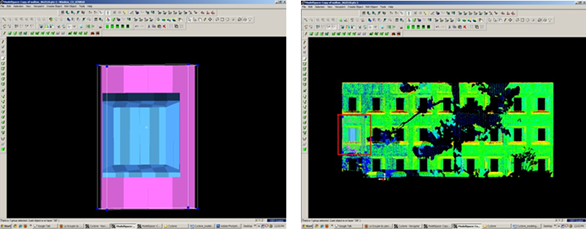
Figure 15 – (Left) Complex feature is grouped and copied (Right) Feature is pasted into the working ModelSpace – note that the feature inserts into the correct position based on the original scan data

[/wptabcontent]

[wptabtitle] DEFINE A “COOKIE CUTTER”[/wptabtitle]

[wptabcontent]

5. If the repeating feature requires a repeating opening, draw a polyline on top of the inserted group to define the opening (this polyline will be used as a “cookie cutter” to make subsequent openings in the wall surface; polyline opening should be slightly smaller than the feature to be inserted -> Place cookie cutter polyline on its own layer

6. Use polyline to create opening in primary (wall) patch (follow steps for “Creating Repeating, Identical Openings“) -> this opening now reveals the grouped window within the primary wall surface

Figure 16 – The large magenta rectangle highlights the entire group; the yellow polyline (representing the “cookie cutter” used to create openings in the primary surface) is slightly smaller than the group

Figure 17 – Opening has been made and the grouped window is revealed – note the yellow polyline “cookie cutter” and the group can be copied and repeated on the primary wall patch[/wptabcontent]

7. Select the Window Group and the “cookie cutter” polyline -> Copy to the next location; there are several methods for placing the repeating feature; two possibilities are outlined below, however different options can be mixed/matched:

7A. Copying and Locating by Pick Points > Multi-select 1st) Group/window 2nd) cookie cutter polyline 3rd) Point representing location where copied object is to be placed -> Create Object -> Copy

7B. Copy dialogue box appears and points that have been chosen are numbered -> Direction of Move, click on blue arrow -> Point to point, define points to use for direction of move and ok -> Distance of move, click on blue arrow -> Point to point, define points to use for distance and ok -> At main dialogue, confirm objects are correctly identified in the “Apply To” pull-down menu -> Copy

Note: If pick points do not show up correctly when copy dialogue box appears, you can re-define pick points while copy command is active; simply multi-select new pick points before defining direction and distance

Figure 18 – Window Group and Polyline are copied with Cyclone’s green arrow showing direction of copy – note that in this case, both the direction and the distance of the copy are from Point 7 to Point 8

[wptabtitle] MULTIPLE COPIES BY DISTANCE AND AXIS[/wptabtitle] [wptabcontent]

7C. Multiple Copies by Distance and Axis > Multi-select points representing 1st) the starting location of the object to be copied 2nd) the offset distance the object will be copied to -> Tools -> Measure -> Distance -> Point to Point -> Annotation showing distance appears

7D. Continue multi-select command -> Select Object(s) to be copied -> Create Object -> Copy -> Direction of Move -> Choose Axis and ok (arrow appears showing which axis will be used for the copy – note that the direction copy is placed along axis is defined by a positive or negative number in the distance)

7E. Distance of move -> Custom -> Enter amount derived with measure command and ok (a negative or positive possible determines the direction on axis) >Main Copy Dialogue box -> Enter Number of copies – note that copies will be offset from each succeeding copy, NOT from the original start location -> Confirm command applied to objects correctly -> Copy

NOTE: Any error will increase as distance increases; therefore it’s important that you examine each copy for accuracy and manually adjust as needed, especially those copies at the greatest distance from the original

Figure 19 – Multiple copies (highlighted in magenta) are offset from one another; openings can be seen in the green, point cloud data – note that as distance increases from the original left group, the error between the proposed opening/group and the accurate opening in the point data also increases and must be adjusted[/wptabcontent]

[wptabtitle] REFINING THE PLACEMENT OF REPEATING FEATURES[/wptabtitle]

[wptabcontent]8. Refining the placement of Repeating Features – as noted, small errors in distance increase with repetition/distance. Using the point cloud and the constraints in Cyclone are essential to accurately placing and locating features. In this example, the primary patch (the wall) is located along the x-axis. As succeeding windows become mis-aligned with the actual point cloud openings, windows are adjusted individually to rectify the model with the point data.

For distance moved, specific points are used – in this case the window sill protruded creating a discernible corner to match with the model’s sill corner.

Direction moved is restricted to the x-axis – this ensures that (1) the succeeding windows stay horizontally aligned with the original and (2) all windows stay along the same plane (the main wall where original window was placed).

Note: Surfaces are very rarely perfectly orthogonal and flat; rather they usually have fluctuations and they deviate from perfect angles. As such, when comparing a flat surface that has been modeled to the point cloud data, points should appear dispersed on both sides of the plane/patch; all points should not be completely located on one side or the other as this indicates the plane is not directly referencing the points.

Figure 20 – (Left) A window is misaligned with the point cloud data; zooming in allows the user to use the points very precisely; movement by picking points allows accurate placement of specific features, such as corners, while moving by a standard axis allows orthogonal alignment with other objects, planes, and references (Right) Window is rectified with the x-axis and specific points on the window sill. Note that the visibility of the primary patch (the main wall) has been turned off for clarity of other layers.[/wptabcontent]

[wptabtitle] MISSING DATA AND COMBINING RESOURCES[/wptabtitle]

[wptabcontent]9. Missing data and combining resources – While point cloud data and axes help accurately place most features, in some cases data is simply not present. In these cases, utilizing other resources is essential to creating a complete model that is as accurate as possible. In this example, a tree left a large shadow in the wall and placing windows within this shadow becomes difficult with point cloud data alone.

Utilizing measurements – finding the average distance between other windows and placing the windows in shadow at this offset helps place the windows fairly accurately.

Comparing the model with the photographic data collected during scanning further assists in accuracy.

[/wptabcontent]

[wptabtitle] CREATE OPENINGS IN PRIMARY WALL PATCH[/wptabtitle] [wptabcontent]10. Once each group has been evaluated and placed accurately -> use the cookie cutter polyline to create openings in the primary wall patch as shown in Step 5 of this section -> Erase or hide the polylines as needed once used (erase if merging back into the original ModelSpace and lines are no longer needed; hidden if copying into original ModelSpace and you want to maintain reference objects in the working ModelSpace).

Figure 21 – (Left) Windows, in dark blue, have been individually analyzed and adjusted for accuracy with the point cloud, in green (Right) Openings have been made in the primary wall patch, in light blue; the dark blue window groups are revealed.

[/wptabcontent] [/wptabs]

Posted in Uncategorized, Workflows | Tagged Cyclone, Leica, mid-range scanning, Scanning, scanning range >5 meters, scanning res 1-20+ centimeters

Leica Cyclone 7.0: Advanced Guide for Building Modeling: Modeling a Complex Shape

This series will show you advanced modeling building modeling techniques using Leica’s Cyclone.
Hint: You can click on any image to see a larger version.

As objects become more complex, using layers (Shift + L) becomes essential to organizing and controlling the model space.

[wptabs style=”wpui-alma” mode=”vertical”]
[wptabtitle]MODELING AN ANGLED WINDOW OPENING [/wptabtitle]

[wptabcontent]

A. Modeling a Complex Shape – An Angled Window Opening

Copy area to be modeled into new, working ModelSpace
Familiarize yourself with the object and the different layers/depths in space that you are working with; when angles are involved it’s good to understand where each angle terminates.

Figure 8 (Left) Complex window to be modeled (Right) Familiarize yourself with the layers of space to be modeled – here yellow represents the farthest plane (the glass) and orange represents the closest plane (the wall in which the window is set)
[/wptabcontent]

[wptabtitle]DIVIDE INTO SUB-SELECTIONS IF NESSCEARY[/wptabtitle]

[wptabcontent]

3. It may be useful to divide the point cloud into sub-selections based on their depth in space or on separate areas to model – Rotate the object to view it from the side or top view -> fence the area to be subselected -> RC -> Point Cloud Subselection -> Add Inside Fence

Figure 9 – Point cloud is sub-selected into several clouds based on their depth in space

[/wptabcontent]

[wptabtitle] MODEL THE OBJECT[/wptabtitle]

[wptabcontent]

4. Model the object using patches, extensions and extrusions as previously outlined – when modeling angled or complex surfaces, patches can be created several ways. When fencing an area and fitting a patch, fence the area that best represents the surface – exclude areas where the surface becomes skewed or extreme near boundaries, curves, etc.

5. While snapping adjacent patches together and extending them, extra handles are often created. It’s best to clean up the patches as you go of any extra handles/geometries to maintain simple, clean lines where possible: Select Patch -> ALT + RC on extra handle -> handle removed

Figure 10 – (Left) Extra handles have been created where the patches intersect (Right) Extra handles deleted, leaving the cleanest, simplest geometry possible

[/wptabcontent]

[wptabtitle] MODELING TIPS[/wptabtitle] [wptabcontent]

6. As objects become more complex and angles become more complicated, it may be helpful to visually clarify and define the objects. This can be done several ways, including editing object colors and creating lines along the edges of objects that are intersecting. Lines create crisp edges and create wireframe objects for export later.

6A. Change Object Color -> Select Object -> Edit Object -> Appearance -> Choose color

6B. Creating Lines where objects intersect: Once the patches/objects have been extended to one another > Mult-select 2 intersecting patches -> Create Object -> From Intersections -> Curve (Note that in Cyclone, a curve here is a line. Also note that sometimes lines will extend beyond the object. Select the line -> slide the handles so beginning and end of line is within the object -> use handles or extend command to make the lines form corners) NOTE: It’s recommended to place lines/polylines on their own layer to aid in there selection and visibility later.

[/wptabcontent]

[wptabtitle] MORE MODELING TIPS[/wptabtitle] [wptabcontent]

7. While modeling complex objects, you will encounter areas where surfaces exist but there is no point cloud data to model directly from. Extruding and extending will often produce these surfaces but sometimes creating polylines and customized patches may be the best way to model these areas. Using the handles of previously modeled objects helps maintain the accuracy of the scan data.

7A. Align view to see the vertices of existing objects to use as guides for the edges of the proposed patch.

7B. Choose handles/points to create the new patch – select the points in the order you wish to draw the polyline that will define the edges for the patch. Do not close the polyline, leaving the last line segment open.

7C. Create Object -> From Pick Points -> Polyline -> Assign Polyline to its own layer

7D. Create Object -> From Curves -> Patch

Figure 11 – (Left) Objects have been created from point cloud however no data exists for the area inside the red rectangle (Right) Handles of the previously modeled objects are used as pick points to
define the edges of the custom patch – note that the final side of the polygon is left open

Figure 12 – Polyline that was formed from pick points is used to create new custom patch[/wptabcontent]

[wptabtitle] GROUPING[/wptabtitle] [wptabcontent]

Helpful Hints –

Grouping: Whether repeating a complex feature or using it only once, it’s a good idea to group the various objects together to maintain the integrity of the individual objects and their intersections. Both small and large ScanWorlds can be best controlled through:

(1) Copying specific areas to a new ModelSpace to model individually > Fence > RC > Copy to new MS

(2) Grouping complex features after they are modeled > Select All Objects that compose complex feature -> Edit -> Group

NOTE: Select all objects, NOT points in the grouping; Items may be ungrouped and removed from groups through the same command

[/wptabcontent]

[wptabtitle] HINT – VISIBILITY AND SELECTABLITLY[/wptabtitle] [wptabcontent]Hints

Visibility and Selectability – As complexity increases the use of layers becomes crucial. You can control which layers are visible and selectable in the layers dialogue box during an active command; this becomes very useful as points, objects, and lines become placed on top of one another)

Figure 13 – Magenta highlights the column showing whether layer is visible; yellow highlights the column showing whether layer is selectable – these attributes can be toggled as needed during active commands[/wptabcontent]

[wptabtitle] HINT – ACTIVE COMMAND[/wptabtitle] [wptabcontent]Hints

Active Command Dialogue – The command dialogue at the bottom of the screen is also very useful as models become more complex. It lists everything that is selected (line, point cloud, group, etc), and as each item is selected, the dialogue shows the layer of and the specific coordinates of each

Figure 14 – The dialogue line at the bottom, left of the screen shows information about the items that are actively selected.[/wptabcontent]

[wptabtitle] HINT – EXPLODE COMMAND[/wptabtitle] [wptabcontent]Hints

Explode Command – When a volumetric object is used or when a patch is exploded, it may be necessary to break the volume into individual planes –> Select Object -> Create Object -> Explode[/wptabcontent]

[wptabtitle]CONTINUE TO…[/wptabtitle]

[wptabcontent] Continue to Modeling and Placing Repeating Features [/wptabcontent] [/wptabs]

Posted in Uncategorized, Workflows | Tagged Cyclone, Leica, mid-range scanning, Scanning, scanning range >5 meters, scanning res 1-20+ centimeters

Guide to leveling and aligning the Breuckmann tripod and SmartScan HE for calibration

This workflow will show you how set up the Breuckmann Tripod and SmartScan HE for calibration prior to beginning your scanning project. Hint: You can click on any image to see a larger version.

[wptabs style=”wpui-alma” mode=”vertical”] [wptabtitle] TRIPOD LEGS SETUP[/wptabtitle]

[wptabcontent]
Start with the tripod in the closed position (all three legs together) and check that the legs are the same length, adjusting them if necessary.

Fig. 1: The brackets at the bottom and center of the tripod legs should be at the same level when the legs are closed, and all the feet should touch the floor at the same time.

Open the tripod legs by loosening the wingnut on the central pole of the tripod and sliding the legs outward. Create a wide triangular base with the tripod legs and tighten the wingnut.[/wptabcontent]

[wptabtitle]PLACE TRIPOD NEXT TO TABLE[/wptabtitle]

[wptabcontent]Place the tripod so that two adjacent legs are flush and parallel with the edge of the table or desk on which you have placed (or will place) the calibration chart.

Fig.2: Tripod feet are level and flush with the base of the desk

Fig.3: The lowest bubble level

If you are uncertain about which leg to adjust first, imagine drawing a line down the middle of each leg of the tripod extending through the bubble level. The line that passes closest to the center of the bubble is the leg you should adjust first. In this illustration where A, B and C mark the positions of the legs you should begin by adjusting leg C. To make the bubble move toward the center, level circle, leg C should be lengthened.

Fig.4: To move the bubble toward you parallel to any leg of the tripod, lengthen that leg. To move the bubble away from you, shorten that leg.

Continue adjusting the length of the legs following this logic until the tripod base is level.
[/wptabcontent]

[wptabtitle] ADJUST TRIPOD HEIGHT[/wptabtitle]

[wptabcontent]

5. Set the height of the tripod head so that it is roughly level with the center of the calibration chart by flipping out and then turning the handle, as shown below.

Fig.5: The central pole height is adjusted by turning this handle.

[/wptabcontent]

[wptabtitle] LEVELING TRIPOD[/wptabtitle]
[wptabcontent]6. Next, you want to adjust the tripod so that the second lowest level bubble is also within its level circle. This step is a little fiddly. The second level bubble essentially accounts for any deviations from level between the central pole, the bracket which attaches it to the tripod legs, and the tripod head. The goal is for the central pole to be just that – centered in the middle of the tripod base. Begin by checking that the tripod head is seated flat on the central pole. Loosen the two wingnuts that lock the position of the central pole. Shift the position of the central pole until the level bubble is within the circle and tighten the wingnuts. Be sure to check that this bubble is still indicating the tripod head is level after you attach the scanner to the tripod!

Fig.6: The tripod head.[/wptabcontent]

[wptabtitle] LEVEL TRIPOD 2- LOWEST ADJUSTMENT KNOB[/wptabtitle]

[wptabcontent]7. Use the lowest adjustment knob to align the front edge of the scanner attachment plate parallel to the edge of the desk or table. On the CAST tripod, this should be approximately at the 30° mark on the bottom dial.

8. Finally, adjust the tripod head so that the top bubble is centered in the inner circle of the bubble level. The highest adjustment knob moves the scanner attachment plate along its long axis, the second highest adjustment knob moves the scanner attachment plate along its short axis.

Fig. 7: Tripod head adjustment guide.

Fig. 8: The top bubble level.
[/wptabcontent]
[wptabtitle] LEVEL TRIPOD 3- SIDE DIALS[/wptabtitle]

[wptabcontent]In addition to the top level bubble, you can use the two side dials as guides for setting the level of the tripod head. On flat ground both these dials should read approximately 0°. There is a small silver dot above each dial marking the 0° position.

Fig.9: Side dials on the tripod head.[/wptabcontent]

[wptabtitle] COARSE ADJUSTMENTS[/wptabtitle]

[wptabcontent](left) Quick, coarse adjustments are made by twisting the ‘quick grip’ and then pivoting the tripod head. Be careful using the ‘quick grip’ if the scanner is already mounted on the tripod head, as the uneven weight of the scanner can cause it to pivot faster than you might expect. (right) Fine adjustments are made by twisting the knob below the ‘quick grip’.

Fig.10: Quick grip and fine adjustment positions on the adjustment handles of the tripod head.[/wptabcontent]

[wptabtitle] FINAL CHECK[/wptabtitle]

[wptabcontent]9. After you have leveled the tripod, attach the scanner and check and adjust the level if needed. At this point you should only need to make fine adjustments.

Fig. 11: The scanner mounted on the level tripod.[/wptabcontent]

[wptabtitle]SCANNER SHEET IN SCANNER CASE[/wptabtitle]
[wptabcontent]
10. Once the scanner is positioned, put the chart placement guide on the table. Position the guide so its short edge is parallel to the edge of the table, and the side reading “SENSOR ” is pointed toward the scanner. Check the datasheet for the correct distance between the scanner and the center of the chart placement guide (approximately one meter). The datasheet and chart placement guide are stored in the lid of the scanner’s case.

Fig.12: The datasheet and chart placement guide in the scanner case.
[/wptabcontent]

[wptabtitle]CHART PLACEMENT[/wptabtitle]
[wptabcontent]
11. Place the Chart over the placement guide and center it. There is a screw in the center of the chart’s frame. This screw should be directly over the center line of the chart. You will probably want to use a
straight edge to ensure the calibration chart is parallel and flush with the center line on the placement guide.

Fig. 13: Aligning the calibration chart to the chart placement guide.

When everything is aligned, tape the chart placement guide to the table so it won’t move as you shift the calibration chart.

12. Alignment and leveling is complete!

13. You may now proceed with the calibration. (You may make some further fine adjustments to the height of the scanner and position of the chart once you have activated the lasers and live screen in the calibration.)
[/wptabcontent]

[wptabtitle] CONTINUE TO…[/wptabtitle]

[wptabcontent]
Continue to Section XXXXXX

[/wptabcontent]

[/wptabs]

Posted in Breuckmann HE, Hardware, Scanning, Setup Operations | Tagged Breuckmann, OPTOCAT, Sensor's and Software, Workflow

Leica Cyclone 7.0: Advanced Guide for Building Modeling: Modeling Openings in Objects

This series will show you advanced modeling building modeling techniques using Leica’s Cyclone.
Hint: You can click on any image to see a larger version.

[wptabs style=”wpui-alma” mode=”vertical”]

[wptabtitle] SELECT OBJECT[/wptabtitle]

[wptabcontent]
Note that restoring the original points that are removed when an object is created is essential to placing openings or to creating more complex features within an object.

I. Select Object –> Right Click –> Insert Copy of Object’s Points. Also note that if/when the working ModelSpace is merged back into the original ModelSpace upon closing, all objects and points are merged so any re-inserted points should be considered (most likely deleted) before merging into the original MS.

II. Once the points have been inserted, Align View so that object being modeled is perpendicular to screen (see GMV Guide ‘Model a Non Rectangular Patch’). There are several methods to creating openings, depending on their geometry and whether the opening is repeated:[/wptabcontent]

[wptabtitle] CREATING A SINGLE OPENING[/wptabtitle]

[wptabcontent]

A. Creating A Single Opening:

1. Create primary patch/wall in which hole is to to be made

2. Select Object –> Right Click –> Insert Copy of Object’s Points.

3. Create Fence that is completely inside intended opening

4. Select the primary patch -> Edit Object -> Patch -> Subtract

Figure 5 (Left) Primary Patch with copy of points inserted and fence drawn- note the fence for the proposed opening is completely within the patch; (Right) Fenced area subtracted from primary patch

[/wptabcontent]

[wptabtitle] CREATING AND REPEATING IDENTICAL OPENINGS[/wptabtitle]

[wptabcontent]

B. Workflow for Creating Repeating, Identical Openings:

Create primary patch/wall in which opening is to to be made
Select Object –> Right Click –> Insert Copy of Object’s Points.
Multi-select points to outline the intended opening -> Create Objects -> From Pick Points -> Polyline (Recommendation: Assign this polyline to a new layer to make it easier to use later)
RC -> Fence -> From Selection
Select Primary Patch -> Edit Object -> Patch -> Subtract
Select Polyline -> Select handle + CTRL to move to next location -> Repeat Steps 1-6 (Note the polyline can be edited by using the handles if succeeding openings differ)

Figure 6 Polyline is created from points and placed on its own layer on the first of a series of identical openings

[/wptabcontent]

[wptabtitle] EXAMPLE[/wptabtitle]

[wptabcontent]

Figure 7 (Left) First opening has been subtracted from the primary patch and the polyline has been moved to the second proposed opening; (Right) Identical second opening has been subtracted

[/wptabcontent] [/wptabs]

Posted in Uncategorized, Workflows | Tagged Cyclone, Leica, mid-range scanning, Scanning, scanning range >5 meters, scanning res 1-20+ centimeters

Aligning Data in OptoCAT

[wptabs style=”wpui-alma” mode=”vertical”]
[wptabtitle] Unaligned Scans[/wptabtitle] [wptabcontent]Aligning scans in OptoCAT is done during the data collection process. Once you have collected two scans they will appear un-aligned in the data volume. You will automatically be re-directed to the ‘Align data’ module. OptoCAT will not allow you to proceed until you have aligned the datasets.

[/wptabcontent]

[wptabtitle] Point Picking[/wptabtitle] [wptabcontent]To align the scans pick matching points on each dataset. The point matching algorithm is fairly robust so you don’t have to be too careful.

[/wptabcontent]

[wptabtitle] Re-alignment[/wptabtitle] [wptabcontent]If you are unhappy with the alignment at any point you can revise the alignment of individual datasets by going to the ‘pre-align’ module and picking points as you would during the scan process.

[/wptabcontent]

[wptabtitle] Activate or Deactivate Data[/wptabtitle] [wptabcontent]To limit the number of scans visible in the data volume you can activate or deactivate them by right clicking on them in the project directory.

[/wptabcontent]

[wptabtitle] Aligned![/wptabtitle] [wptabcontent]Once you are satisfied with your alignment, you can push the ‘align’ button to refine before proceeding with further processing.

[/wptabcontent]

[/wptabs]

Posted in Opticat, Workflow | Tagged Breuckmann, close range scanning, OPTOCAT

Leica Cyclone – Creating a Mesh and Modeling Surface Topography: Creating the Topographic Mesh

This series will show you how create a mesh and model surface topography in Leica’s Cyclone
Hint: You can click on any image to see a larger version.

[wptabs style=”wpui-alma” mode=”vertical”] [wptabtitle] SELECT POINTS[/wptabtitle]

[wptabcontent]9. Select Points (when dealing with large areas, selecting several points results in more surface points being sampled in the surface growing process) -> Create Object -> Region Grow -> Smooth Surface -> Cyclone runs the region grow by default settings to show the initial view and the dialogue box – Adjust Surface Characteristics and click ‘Restart’ to preview results -> Click OK when satisified with preview:

Hardtop Surface (this is generally chosen for fairly uniform areas with paved or hard surfaces; if dealing with rolling unpaved terrain, uncheck this option).Viewing the point cloud with color from scanner or hue intensity is recommended for this process Per Cyclone 7.0 Glossary: “This command is used to segment a selected smooth surface in a point cloud. The points representing the smooth surface are merely segmented from the point cloud; no object is inserted. This command is not available for use with a pcE file (pcE cloud).”

[/wptabcontent]

[wptabtitle] DECIMATE AND SUBDIVIDE[/wptabtitle]

[wptabcontent]10. Decimate Mesh (per Leica Trainer July 2010 current bug in meshing command) -> Select Mesh -> Tools -> Mesh -> Decimate -> Maintain 100% of original triangles, vertices, and exact boundary edges -> Decimate allows pre-view -> OK to accept

11. Subdivide areas by breaklines -> Select Boundary Breaklines and Mesh -> Tools -> Breaklines -> Extend Polylines to TIN -> (NOTE: This command extends a polyline onto a TIN ojbect, creating edges in the mesh based on the projection of the polyline vertically onto the mesh – although polyline itself does not change. The edges are stretched vertically to conform to the polyline’s shape – If select command through Breaklines submenu, polyline will be converted to breakline on the mesh; if select command through polyline submenu, resulting line will be a geometric object

NOTE: If errors appear:(1) Select Mesh -> Tools -> Mesh -> Verify TIN -> If TIN is not valid, the number of invalid faces will be listed and the faces will be selected -> Tools -> Mesh -> Delete Selection -> Repeat this verfication and deletion process until TIN successfully verified; (2) If errors regarding polylines overlapping -> Select Polylines -> Tools -> Drawing -> Align vertices to axes

[/wptabcontent]

[wptabtitle] ADDITIONAL STEPS[/wptabtitle]

[wptabcontent]12. Re-insert break lines (copied in Step V) -> Copy from temporary location -> Paste into working mesh MS

13. Editing Triangles and Spikes -> In layers dialogue box -> View As tab -> Apply to Mesh -> Wireframe -> Apply & OK ->

14. In top view, fence in problematic triangle(s) causing spike -> Fence -> Delete Inside -> Select hole (highlights cyan) -> RC -> Mesh -> Fill selected hole[/wptabcontent]

[wptabtitle] EXPORTING[/wptabtitle] [wptabcontent]15. Exporting 3D Lines, Mesh, Point Cloud -> There are several options for exporting topographic features.The objects created through tracing and meshing can be exported or the point cloud itself can be exported.

A. Export the lines, polylines, arcs -> Use the properties manager (Shift + L) to turn off the visibility/selectability of the point cloud -> Select All -> File -> Export

DXF R12 Format –This retains 3D information (in this case the z-coordinate for the lines); Do not select 2D DXF R12 Format

Objects may also be exported as ASCII or XML file types here

Once exported, the .dxf file can be opened in CAD, imported into Sketchup, or converted for use in multiple software.

B. Export the mesh -> Select mesh -> File -> Export -> Select file type for destination software

C. Export the Point Cloud -> Newer versions of Autodesk products (2009 and beyond) support point clouds.If you do not have Cyclone but you do have CAD, use Cyclone to export the points and then trace/model in CAD software much as we have done in Cyclone.The main issue is file size when importing into CAD; in general, point clouds must be broken into smaller pieces to allow them to be imported.See the CAST workflow, ‘Reducing Point Clouds for Autodesk Applications’ for more details.

NOTE: In general, a .PTS file with a maximum size of 4mb will import into CAD

Create new layers for the breaklines and features (Shift + L) -> Review the area to be modeled identifying where the surface changes and/or where the user wants a clean break or difference between adjacent surfaces.Create layers for primary and secondary features as needed.

[/wptabcontent] [/wptabs]

Posted in Uncategorized, Workflows | Tagged Cyclone, Leica, mid-range scanning, Scanning, scanning range >5 meters, scanning res 1-20+ centimeters

Using Leica’s COE Plug-in in Cyclone

This workflow will show you how to use Leica’s COE plug-in to import and export objects and points in Cyclone.
Hint: You can click on any image to see a larger version.

[wptabs style=”wpui-alma” mode=”vertical”] [wptabtitle] IMPORTING & EXPORTING[/wptabtitle]

[wptabcontent]

Importing & Exporting Objects and Points in Cyclone with COE Files

I. Importing files into Cyclone is done through the Navigator window, where a new MS is created with the imported file -> Open Cyclone Navigator -> Select Database/ModelSpaces Folder -> RC -> Import -> browse to COE file -> Open -> MS View appears named by default with the COE file location

NOTE: You cannot import a COE into a MS view, rather it must be imported into the overall “ModelSpaces” project folder at which time a new MS view is created for editing. While most objects can be imported into Cyclone, complex objects (ie: beveled edges, rounded corners, notches) may be translated into a collection of lines and arcs versus objects when imported

[/wptabcontent]

[wptabtitle] MANAGING THE COE-MS[/wptabtitle]

[wptabcontent]II. Managing the COE-MS -> Open the COE ModelSpace that has automatically been created -> It is recommended that you group objects and place them on individual layers as needed in this original COE MS (to group -> Select Objects -> Edit -> Group -> Group -> Objects can be ungrouped at any time with this command as well) -> Copy all objects -> Close COE MS[/wptabcontent]

[wptabtitle] PASTING COE OBJECTS INTO ORIGINAL MS[/wptabtitle]

[wptabcontent]III. Pasting COE objects into Original MS -> Its highly recommended to copy and paste the original MS as a copied/working MS in Cyclone Navigator; use this copied MS to insert objects, updating the original MS only as a final step -> Open copied MS -> Paste objects that were copied from COE file in Step II -> NOTE: if coordinates were maintained and referenced throughout the modeling and export process, the object should automatically paste into the correct position. If references/links have been lost, the imported objects may need to be moved/rotated (select objects -> RC -> move/rotate)

NOTE: When moving grouped or multiple objects, faces and lines may appear to remain in their original position or become displaced during manipulation; as long as all objects are selected or grouped/selected, this is only a refreshing issue -> View Properties (Shift + L) -> Selectable/Visible Tab -> toggle the visibility of the object type off (ie: mesh or patch, etc) and when toggled back on, the view of all objects should be refreshed.

[/wptabcontent]

[wptabtitle] COMPARING MODELED OBJECTS WITH ORIGINAL POINTS[/wptabtitle]

[wptabcontent]

Comparing Modeled Objects with Original Points in Cyclone

I. Import the COE file into Cyclone Navigator

II. Upon importing, the COE creates its own MS that loses many of the editing/manipulation options -> Open the COE MS -> Select All -> Copy -> Open Working MS (containing points to compare/analyze) -> Paste COE object(s) into Working MS; NOTE: Pay attention to the layers in Cyclone: all ACAD layers accompany the object when imported however when copied/pasted objects are placed on a layer named ‘default~’; Manually assign the correct layer to the object in the Working MS and delete unnecessary layers.[/wptabcontent]

[wptabtitle] CALCULATE MESH TO POINT CLOUD DEVIATION[/wptabtitle] [wptabcontent]III. Calculate Mesh to Point Cloud Deviation -> Multi-select the object mesh and the point cloud (Its recommended to view the mesh in “per-face normals” setting > Shift + L for Layers > View As tab) -> Tools -> Measure -> Mesh to Points Deviation -> Dialogue Box Options:

Slider bar allows user to adjust and preview deviations on the mesh faces above a user-set limit; minimum and maximum boxes are read-only
Distance computation – user decides whether those faces that are highlighted are based on maximum or average deviation and Absolute (no positive/negative distances) or Signed Distance
Details – displays total mesh faces, # of faces deviating, what percentage of the whole that represents, and total # of points

[/wptabcontent]

[wptabtitle] CALCULATING DEVIATION – CONT.[/wptabtitle] [wptabcontent]IV. Calculate Object to Point Cloud Deviation when Object is created in Cyclone > Object (ie: cylinder, primitives) -> after creation, select object and RC -> Info dialogue tells Fit Quality including Error Mean, Error Std. Deviation, and Absolute Errors; Interfering Points may also be calculated

V. Calculate Object to Point Cloud Deviation when Object is created outside of Cyclone -> Interfering Points -> Multi-select object and point cloud -> Tools -> Measure -> Interfering Points -> Dialogue box appears in which user can adjust the tolerance to calculate -> all cloud points that are within the user-specified distance of the selected object are highlighted and can be segmented from the rest of the cloud (See Cyclone help ‘How to Segment interfering points’ for more details) and dialogue box displays the percentage of points interfering and the percentage of points inside the object (useful in volumes); this analysis is limited in many modeling applications as accurately modeled objects rarely lie completely on one side of the points referenced

[/wptabcontent] [/wptabs]

Posted in Leica CloudWorx, Uncategorized | Tagged Cyclone, Leica, mid-range scanning, Scanning, scanning range >5 meters, scanning res 1-20+ centimeters

Modeling an Irregular Features – Comparing Modeled Objects to Original Points

In this series, columns in a deteriorating colonnade will be modeled by several methods.
Hint: You can click on any image to see a larger version.

[wptabs style=”wpui-alma” mode=”vertical”]

[wptabtitle] CLOUDWORX[/wptabtitle]

[wptabcontent]

Comparing Modeled Objects to Original Points in this example

(analyzed at .005 m (.5 cm) / average distance of deviation/ absolute value)

I. CloudWorx – three section cuts in the x or y direction – lofted in the z (up) direction to create 3D solid column:

· 7% of the mesh faces (ie: 484 of 6,914) were above .5 cm deviation from point cloud

[/wptabcontent]

[wptabtitle] CLOUDWORX 2[/wptabtitle]

[wptabcontent]

II. Cloudworx – 1 section cut in the z direction (representing 1/2 the column from outside edge to center) – revolved around center axis to create 3D solid column

· 43% of the mesh faces (ie: 6,055 of 14,160) were above the .5 cm deviation from point cloud

[/wptabcontent]

[wptabtitle] CYCLONE[/wptabtitle]

[wptabcontent]

III. Cyclone – Mesh created in Cyclone from point cloud

· < 1% of the mesh faces (ie: 977 of 334,133) were above the .5 cm deviation from point cloud

[/wptabcontent] [/wptabs]

Posted in Leica CloudWorx, Uncategorized | Tagged CloudWorx, Cyclone, Leica, mid-range scanning, Scanning, scanning range >5 meters

Modeling an Irregular Features – Method 2

In this series, columns in a deteriorating colonnade will be modeled by several methods.
Hint: You can click on any image to see a larger version.

[wptabs style=”wpui-alma” mode=”vertical”] [wptabtitle] USE THE CLOUDWORX SLICE TOOLBAR[/wptabtitle]

[wptabcontent]Method 2: Slicing Single Cross Section and Revolving the Profile Around Center – Similar to the first method, the column will be sliced and traced; however here, a single profile will be traced and revolved around the center, creating a solid or surface object. Follow steps in Method 1, Section I for setting up the ACAD model space and isolating the colonnade.

I. Use the CloudWorx Slice Toolbar to slice the point cloud from the top view (or whichever view allows you to see the entire diameter of the column/feature); this will be the only section profile that will be traced and we will only be tracing half of it; choosing the most complete/intact slice possible is recommended. See Method 1 for details on slicing

Figure 7 (Left) Top view of the column; magenta lines highlight the slicing boundaries – (Center) Top view of the column profile slice – (Right) Front view of the column profile slice

[/wptabcontent]

[wptabtitle] TRACE THE PROFILE AND SNAP TO POINT CLOUD[/wptabtitle]

[wptabcontent]

II. Trace the profile of the section cut, snapping directly to point cloud > Front or Side View > Make correct layer current > Zoom in to view points comfortably and refresh point cloud to confirm all points visible (do this periodically, especially when zooming in/out) > Command Line: PL or POLYLINE and begin to trace the profile/outline the profile of the section cut

REMEMBER: (1) Enable OSNAP “NODE” to snap to points (2) At command line: type “U” during active polyline command to undo vertices/go back without ending the command (3) At command line: PEDIT allows polyline(s) to be edited, joined, etc. (4) See ACAD Help: Drawing and Editing Polylines for more information

[/wptabcontent]

[wptabtitle] DETERMINE CENTER AROUND WHICH TO ROTATE[/wptabtitle] [wptabcontent]III. Determine the center around which to rotate > NOTE: there are a variety of ways to determine the center of a feature; one is outlined here. Also see the “fit pipe to cloud” method (following section), which determines the center directly from the point cloud and places a polyline along the centerline >

A. After half of the profile has been traced turn on ORTHO mode, which restricts drawing to a 90-degree vertical and horizontal direction to ensure clean angles for the rotation later

B. OSNAPS – enable ENDPOINT and MIDPOINT -> Use ONSNAPS to draw a line that is perpendicular to the column’s profile polyline: the start point snaps to the endpoint of the top of the column and the end point snaps to the point cloud on the opposite edge of the section cut – this line represents the full diameter of the column. Draw another line in the same way at the bottom of the column (See Figures 12 & 13)

Figure 8 (Left) Front view of point cloud and polyline representing left profile of the column – (Center) Front view with the point cloud hidden – (Right) Original polyline with perpendicular lines drawn at the top and bottom representing the diameter of the column

[/wptabcontent]

[wptabtitle] EXAMPLES[/wptabtitle]

[wptabcontent]

Figure 9 – Front view, close-up of the top of the column; on the left of the image, the yellow polyline is the original line tracing the point cloud profile (dense green points). With osnaps, draw a line snapping to the end point of the original polyline. Ortho Mode ensures a perpendicular line to the opposite edge of the point cloud/column (less dense green dots on the right side of the image). Repeat this process at the bottom to achieve the 3 lines shown in Figure 8.

[/wptabcontent]

[wptabtitle] USING OSNAPS[/wptabtitle] [wptabcontent]

C. Use OSNAPS to snap to the midpoint of the line at the top of the column to the midpoint of the line at the bottom of the column – this line represents the center of the column (TIP: When snapping to midpoint, a triangle and the word “midpoint” appears near the cursor) -> Use grips or the TRIM command to trim the ends of the lines that protrude past the center line

NOTE: This method finds the center based on the diameter of the column at the top and bottom at the point of the slice, accounting for any leaning/tilting along the z-direction; For generally upright features, drawing a line in the center and restricting it to the z-axis will result in more regularized features with identical “up directions”

IV. Command line: PEDIT to edit the polylines and join them into a single closed polyline > PEDIT > Select original polyline > JOIN > Select centerline, top line, and bottom line > ENTER 2X > Clicking on the polyline should confirm that it is now a single object (if it does not join, check to confirm no endpoints are snapped to one another but they are NOT overlapping).

Figure 10 (Left) Draw a polyline from the midpoint of the top line to the midpoint of the bottom line – note the yellow triangle and ‘midpoint’ showing the OSNAP constraint is active (Right) Polylines have been drawn, trimmed, and joined to form a single polyline representing the profile of the column from the center to the edge

[/wptabcontent]

[wptabtitle] ROTATE PROFILE TO FORM 3D OBJECT[/wptabtitle]

[wptabcontent]V. Rotate profile to form 3D object > Create and make a separate layer for the 3D object and make it active > 3D Modeling main toolbar > EXTRUDE tab pulls down to REVOLVE (see figure 4) or at command line: REVOLVE > select profile polyline > ENTER > “Specify Start point or define axis” > Select endpoint at the bottom of the centerline > “Specify axis endpoint” > Select endpoint at the top of the centerline > “Specify angle of revolution” > ENTER to accept default of 360-degrees

Figure 11 (Left) The centerline of the column is drawn by snapping from the midpoint of the bottom polyline to the midpoint of the top polyline (Right) 2D tracing of the point cloud section cut is revolved around the centerline creating 3D object

6. Modeled object can now be edited or exported as desired.[/wptabcontent]

[wptitle]CONTINUE TO…[/wptabs]

[wptabcontent]Continue to Comparing Modeled Objects to Original Points[/wptabcontent]

Posted in Leica CloudWorx, Uncategorized | Tagged CloudWorx, Leica, mid-range scanning, Scanning, scanning range >5 meters

Leica Cyclone – Creating a Mesh and Modeling Surface Topography: Setting Up the Model Space and Break Lines

This series will show you how create a mesh and model surface topography in Leica’s Cyclone
Hint: You can click on any image to see a larger version.

[wptabs style=”wpui-alma” mode=”vertical”] [wptabtitle] INTRODUCTION AND DEFINITIONS[/wptabtitle]

[wptabcontent]In this guide, a mesh is considered to be a series of triangles that represents a surface. Cyclone generates meshes by using the points in a point cloud, vertices, polylines, or any combination of the three as vertices. For each adjacent trio of points in a cloud, a triangle is created. This has the effect of creating a visually coherent surface from the point cloud, and it is the primary method for modeling topography.

Break lines are lines or polylines that sub-divide the mesh; they represent the edges of a paved surface, a ridge, a channel, or any other topographic feature that the user wants to preserve. While mentioned in 2D topographic tracing, break lines become very important in meshing. Here, they have an accurate z-coordinate and they become the edges that the triangles in the mesh conform to, defining and controlling the smoothness and continuity of the mesh. They allow the user to break-up the mesh into reasonable “chunks” for future texturing and detailing.

Please see ‘Leica Cyclone – Creating a Basic CAD Ojects From Surface Topography (2D)’ as a supplement to this workflow.[/wptabcontent]

[wptabtitle] OPEN A REGISTERED UNIFIED MODEL SPACE[/wptabtitle]

[wptabcontent]1. Open a Registered Unified Model Space -> Create fence around ground plane –> Right Click –> Copy Fenced to new Model Space (NOTE: viewing from a standard side, front, or back view in orthographic mode assists in selection) -> Original MS may be closed

Figure 1 – (Left) Original registered scan world of plaza (Right) Point Cloud Sub-Selection (Select -> Right Click -> Point Cloud Sub-Selection) allows unneeded points, such as trees and vertical surfaces, to be deleted; Sub-selection allows the user to precisely choose and view points before deciding to delete

[/wptabcontent]

[wptabtitle] SELECT AND DELETE UNNEEDED POINTS[/wptabtitle]

[wptabcontent]2. In the new Working MS -> Select and delete unneeded points (it’s best to eliminate as much vertical surface data as possible so that the ground plane to be modeled is isolated; objects in motion, such as trees/vegetation can be especially problematic and cleaning up areas where these are abundant is suggested; eliminating data that may be present inside buildings or areas that will not be modeled is also suggested)

Figure 2 – The same plaza as Figure 1 now copied to a working MS and “cleaned” of unneeded vertical surfaces and vegetation leaving only the ground plane to be modeled.

[/wptabcontent]

[wptabtitle] CREATE NEW LAYERS FOR THE BREAKLINES AND FEATURES[/wptabtitle]

[wptabcontent]

3. Create new layers for the breaklines and features (Shift + L) -> Review the area to be modeled identifying where the surface changes and/or where the user wants a clean break or difference between adjacent surfaces.Create layers for primary and secondary features as needed.

4. Create lines to represent the topography and features, assigning an accurate x, y, and z coordinate -> There are several ways to make lines including (1) using 2D drawing methods (covered in ‘Topography and Site Elements – 2D’ above) (2) with pick points, (3) by extending an existing line (4) by snapping two existing lines together (5) by creating a polyline with Fit Edge command, and (6) by merging polylines together.

See Help -> Contents -> Search -> ‘Make Lines, Polylines, and Breaklines’ for steps for each of these methods.There are additional variations of each.BEWARE: Lines created by pick points cannot be used for break lines in meshing; if picking points, be sure to create a polyline rather than a line segment.[/wptabcontent]

[wptabtitle] TIPS[/wptabtitle]

[wptabcontent]5. Tips

A. If drawn in 2D, use Edit Object -> Move/Rotate to move the object to the correct z-coordinate; there are multiple options moving objects including by a standard axis and pick points.

B. Create additional break lines following the feature or edge of the break lines; place these to break up the mesh and around the boundaries, segmenting out areas where a topographic ground plane is not needed (ie: inside buildings)

Figure 3 – Top view of plaza; Polylines have been created to outline where the sidewalk and grass meet; orange handles help highlight the polylines

[/wptabcontent]

[wptabtitle] MORE TIPS[/wptabtitle]

[wptabcontent]More Tips:

C. Use multiple views to confirm line is properly located at all angles and handle constraints (Edit Object -> Handles constrain to -> Various options – NOTE: once placed in top view, constraining handles to z-direction helps placement in 3D)

D. Try different methods to see what works for you.With all, use multiple views to confirm the line is properly located at all angles

Figure 4 – (Left) Although from Top View, the breakline looks correct, inspection from a different angle reveals that it is not correct (Right) Handles and constraints (Edit Object -> Handles -> Constrain Motion) are used to pull the polyline into the correct position – every section of every breakline should be inspected from multiple views

[/wptabcontent]

[wptabtitle] FINAL STEPS[/wptabtitle] [wptabcontent]6. Create handles at places where polylines intersect (Select line -> ALT + Select point on line for new handle to help snap lines together).

7. Delete all points beyond boundary of mesh -> Select polyline representing boudary of mesh -> Right click -> Fence -> From Selection -> Fence -> Delete outside

8. Delete points within other breaklines to remove any remaining points that should not be considered in the creation of the mesh -> Copy final breaklines to original or temporary working space in case altered/needed in future

8. Unify points reducing spacing to 1 foot to start and adjust settings for desired results.[/wptabcontent]

[wptabtitle]CONTINUE TO…[/wptabtitle]

[wptabcontent]Continue to Creating the Topographic Mesh[/wptabcontent][/wptabs]

Posted in Workflow, Workflows | Tagged Cyclone, Leica, mid-range scanning, Modeling, Scanning, scanning range >5 meters, scanning res 1-20+ centimeters, Workflow

Setting up the Breuckmann SmartSCAN HE

This workflow will show you how set up the Breuckmann SmartScan HE prior to beginning your scanning project. Hint: You can click on any image to see a larger version.

[wptabs style=”wpui-alma” mode=”vertical”] [wptabtitle] FOV[/wptabtitle] [wptabcontent]The SmartSCAN HE is a dual camera white light scanner that uses fringe projection to measure precise 3D coordinates. The unit owned by CAST is a 5 MP(megapixel) system that captures color and includes three lenses or fields of view (FOV): 125mm, 475mm, and 825mm. The field of view measure is the length along the diagonal of the scan-able area (shown in Figure 1 below).

clip_image001

Figure 1: Approximate scan area using 125mm FOV with Breuckmann scanner

A good way to remember the different lens sizes is:

– 125mm: baseball/softball size scan area

– 475mm: basketball size

– 825mm: two basketballs or yogaball size

[/wptabcontent]
[wptabtitle] SIZE OF ARRAY[/wptabtitle] [wptabcontent]The size of the array – 5MP (2448×2048) is static for each of the fields of view. Scanning with the 125mm lens will provide 5,013,504 measurements across the area the size of a softball while scanning with the 475mm lens provide the same number of measurements across the area the size of a basketball. Therefore, a smaller FOV = higher data resolution. The approximate resolution for each of the lenses is provided in the table below:

Breuckmann Lens/FOV	Estimated Data Resolution (in microns)
125	60
475	280
825	500

It is important to choose an appropriate lens for your scan project. The size of the object, the desired resolution, the final product for the project, and the amount of time available to scan are all important factors to consider.[/wptabcontent]

[wptabtitle] SETTING UP THE BREUCKMANN[/wptabtitle]

[wptabcontent]
The Breuckmann setup includes three items: the scanner case(1), the calibration chart case(2), and the tripod(3).

Figure 2: (1) Case containing scanner, optolink, and all necessary cables, (2) Case containing large calibration chart, (3) System tripod

At minimum the scanner case and tripod are necessary for every scan project. It is recommended to calibrate the scanner every time the lenses are changed on the scanner. If you are using the mid (475mm) or large (825mm) FOV’s, then you will need to calibrate the system using the large calibration chart in case #2. The calibration chart for the small (125mm) FOV is in the main scanner case. Please see the workflow on Calibrating the Breuckmann for more information on system calibration.[/wptabcontent]

[wptabtitle] TRIPOD SETUP[/wptabtitle]
[wptabcontent]When setting up the Breuckmann, first setup the system tripod. While it is not required for the tripod to be level for scanning objects, it should be level when performing a system calibration. The tripod that is used has four levels on it (shown below). When leveling the tripod, it is best to first level the very base of the tripod (level#1) and then to level the tripod mount using the very top level (level #2). The other levels are not used.

Figure 2: Tripod levels. Only use levels 1 and 2 when leveling the tripod.

[/wptabcontent]
[wptabtitle] CONTENTS OF CASE[/wptabtitle] [wptabcontent]Next open the Breuckmann case, and remove the large piece of t-shaped foam. The case components are shown in the image below.

clip_image007 Figure 3: Scanner components in main scanner case

[/wptabcontent]

[wptabtitle] PLACING ON TRIPOD[/wptabtitle]

[wptabcontent]Next, remove the scanner from the case and place on the tripod.

IMPORTANT: The lever on the tripod will click into place once the scanner is secured. Do NOT LET GO of the scanner until you have heard the tripod mount click. Also, always use the silver handle located on top of the scanner when moving the scanner from the box to the tripod or vice versa.

clip_image009

Figure 4: Placing the scanner onto the tripod
[/wptabcontent]

[wptabtitle] LENSES[/wptabtitle]

[wptabcontent]
Once the scanner is on the tripod, next choose the appropriate lenses for your project. Each set of lenses include one lens for the left camera, one lens for the right camera, and one lens for the projector. When looking at the lenses, the first set of letters indicate whether the lens is for the left camera (CL), the right camera (CR) or the project (P) and the last set of numbers indicate the FOV (12 = 125mm, 47 = 475mm, and 82 = 825mm). Notice the labels on the set of lenses below for the 825mm FOV.

clip_image011

Figure 5: Set of lenses for the 825mm FOV (CR = Camera Right, P=Projector, and CL = Camera Left)

One set of lenses will already be in place on the scanner. If you have to change the lenses, the additional lens sets are located under the pieces of foam directly under the scanner in the case. Before removing the lenses from the scanner, make sure the orange lens caps are in place and locate the black lens caps in the case that are used for the other side of each lens. Unscrew a lens from the scanner and IMMEDIATELY place the black lens cap on the other side of the lens. Repeat for all lenses and place each lens in the individual pieces of bubble wrap provided in the case. BABY THE LENSES as they are a crucial part of the system and can easily be scratched.

When standing behind the scanner, the projector is the center lens the left camera is to left (and farthest from the projector) and the right camera is to the right (closest to the projector). When installing new lenses it is critical to get the correct lens in the correct location. All lenses should be tightly screwed in.

clip_image013

Figure 6: Camera and projector locations on the SmartSCAN

[/wptabcontent]

[wptabtitle] INTERFACING SCANNER WITH A DESKTOP COMPUTER (IN LAB)[/wptabtitle]
[wptabcontent]
Once the scanner is setup, remove the Optolink (black box) and all necessary cables. The large black cable connects the scanner to the Optolink (via the main connector) and the computer (via two firewire connections). The Optolink has its own power cable and is also connected to the computer (via USB).

clip_image015

Figure 7: Diagram showing connectivity between SmartSCAN, Optolink box, and desktop computer

Connect the main connector to the scanner. Make sure the connection is square and screw in to secure (Note: Screws should go in easily. If not, you might be cross-threading the connection). Each camera has three cables. Be sure and line up the dots on the smallest round connection (1). Plug the remaining cables in accordingly and be sure to screw in the firewire connections using the screwdriver provided in the case. DO NOT FORCE ANY CONNECTIONS!!!

clip_image017

Figure 8: Three camera cables and their associated connections

When plugging cables into the scanner, it is essential to lift the cable slightly and attach it to the scanner handle using the attached Velcro strap. This prevents the weight of the cable from straining the connections.

clip_image019

Figure 9: Completed scanner setup with Velcro strapped secured around handle for support

Next, take the opposite end of the black cable and plug the main connector into the Optolink and the two firewires into the back of the desktop. Again, use the provided screwdriver to secure the firewire connections. Finally, connect the Optolink to the desktop using the brown, reflective USB cable and plug the power cord for the Optolink into an outlet. The scanner and associated hardware are now ready to use. Power the Optolink first and then the computer. You are now ready to open the Optocat software and begin your scan project.[/wptabcontent]

[wptabtitle] INTERFACING THE SCANNER WITH A LAPTOP (IN FIELD)[/wptabtitle]
[wptabcontent]
The Dell M4500 laptop is the currently the only CAST laptop that is configured to interface with the Breuckmann. The Magma box (silver box) is an additional piece of hardware that is required to connect the laptop with the scanner. Remove the Magma box, Optolink, and all associated cables from the scanner case. The difference between the laptop configuration and desktop configuration is that the two receiving firewire cables plug into the Magma box and the Magma box connects to the laptop using a express card adapter.

The large black cable connects the scanner to the Optolink (via main connector) and the magma box (via two firewire connections). The Optolink has its own power cable and is connected to the computer (via USB). The Magma box also has its own power cable and it connected to the computer via an express card adapter that fits into the express slot on the left side of the laptop.

clip_image021

Figure 10: Diagram showing connectivity between SmartSCAN, Optolink, Magma box, and laptop

Connect the main connector to the scanner. Make sure the connection is square and screw in to secure (Note: screws should go in easily. If not, you might be cross-threading the connection.) Be sure and line up the dots on the smallest round connection (1). Plug the remaining cables in accordingly and be sure to screw in the firewire connections using the screwdriver provided in the case. DO NOT FORCE ANY CONNECTIONS!!!

Next, take the opposite end of the black cable and plug the main connector into the Optolink and the two firewires into the Magma box. Again, use the provided screwdriver to secure the firewire connections. Next, connect the Optolink to the desktop using the brown, reflective USB cable and plug in the power cord for the Optolink. Finally, connect the Magma box to the computer using the serial cable and Express Card adapter and plug in the power cord for the Magma box.

clip_image023

Figure 11: Express card adapter that fits the Express card slot on the laptop

The scanner and associated hardware are now ready to use. Power the Optolink and then turn on the computer. You are now ready to open the Optocat software and begin your scan project.[/wptabcontent]

[wptabtitle] BREUCKMANN DISASSEMBLY[/wptabtitle]
[wptabcontent]
Disassembling the scanner is fairly straight forward with a few notable points. All screwed-in connections including the main connector and all firewires should be unscrewed completely and then pulled. Of the three camera cables, the smallest round connection (1) can be disconnected simply by pulling firmly on metal grips. The large round connection (2) is push-pull connector, so first slide the metal grips forward and then pull to disconnect.

clip_image024

Figure 12: Image showing three cables/connections for each camera

To remove the scanner from the tripod, pull the silver lever on the tripod mount back to disengage the connection and to remove the scanner. Always carry the scanner by the silver handle.

clip_image026

Figure 13: Pull silver lever towards the back of the scanner to remove the scanner from the tripod

Once everything is in the case, double check that all cables/connections are tucked securely in the case before closing the lid.

clip_image028

Figure 14: Successful pack up! (Minus the Magma box)[/wptabcontent] [/wptabs]

Posted in Setup Operations | Tagged Breuckmann, Data Collection, OPTOCAT

Under Construction

This document or link is still being developed. Please check back soon!

Posted in Uncategorized

Leica Cyclone 7.1.1: Sub-Dividing Large Point Clouds for Autodesk Applications – Final Images from Example

This page will show you examples of sub-divided point clouds.
Hint: You can click on any image to see a larger version.

[wptabs style=”wpui-alma” mode=”vertical”] [wptabtitle] TOP VIEW[/wptabtitle] [wptabcontent]VI. Final Images from Example

Figure 16 – Top view of the building with all of the vertical RP’s visible; note the top-most RP (above Piece_001) is the original vertical RP that was created from the wall/patch and defined the direction of the grid and the division

[/wptabcontent]

[wptabtitle] SIDE VIEW[/wptabtitle] [wptabcontent]

Figure 17 – Side view of the building with the single horizontal RP that was used; note that this was the original, default RP that was moved to a point on the floor of the main level.

[/wptabcontent]

[wptabtitle] SIDE VIEW[/wptabtitle] [wptabcontent]

Figure 18 – Side view of the building with all RP’s visible; note that in terms of physical dimensions, the pieces are not identical. The left side of the building is filled with complex layers of pipes – this resulted in more points and density. The RP’s were placed close together making the physical dimensions of Piece_001 smaller than pieces to the right. The right side of the building had larger, less complex equipment resulting in sparser points and density. This meant that the physical dimensions of the pieces were larger although the size of the pieces (# of points) and the size of the exports remained consistent. Finally, note the naming logic, the number indicates it’s from left to right and the letter A or B identifies whether it was the main level or basement level.[/wptabcontent]

[wptabtitle] FRONT VIEW[/wptabtitle] [wptabcontent]

Figure 19 (Left) – Front view of a sectional cut and the horizontal RP used to divide the A & B cuts; Figure 20 (Right) – Perspective view of the same piece; note that initially looking at the data, the lower section has smaller physical dimensions and appears to be less complex/dense. However, the number of points and the size of the export for the top section were approximately equal to the relative sizes of the bottom section. The bottom section was extremely confined with many obstructions and a limited scanning range – resulting in very dense data on objects close to the scanner. The top section was open and the occurrence of very dense data due to proximity to the scanner was much lower. Here the scanning range itself resulted in the need for smaller pieces to achieve the appropriate file sizes.

[/wptabcontent] [/wptabs]

Posted in Cyclone, Scanning, Software, Uncategorized, Workflows | Tagged Cyclone, Leica, mid-range scanning, Scanning, scanning range >5 meters, scanning res 1-20+ centimeters

Z+F Laser Control: Interface Basics

[wptabs style=”wpui-alma” mode=”vertical”]
[wptabtitle] INTERFACE BASICS[/wptabtitle]

[wptabcontent]

Z+F Laser Control Interface Basics

Figure 1: Laser Control Toolbars

[/wptabcontent]

[wptabtitle]VIEWING A SCAN IN 3D[/wptabtitle]

[wptabcontent]

1. To view a scan in 3D, RC in the 2D View and select Points to 3D (this gives you the most options), you can also select Full Scan to 3D (automatically subsamples) or Selection to 3D(automatically subsamples). In the Points to 3D options the Subsample factor is the key element to adjust. The default subsample is 0 which is automatic. If you want to see all of the data, set it to 1 (1/1) if you want it subsampled, set it to 4 (1 point is displayed for every 4) or 8 (1 for every 8). You can also filter by intensity and range and also do basic Mixed Pixel filters here. Remember this only filters that what you SEE in the 3D Window and doesn’t actually filter the data at all.

Figure 2: Points to 3D options

[/wptabcontent]

[wptabtitle]OPTIONS FOR 3D VIEW[/wptabtitle]

[wptabcontent]2. Look at the image for other options in the 3D View. Note: The 3D View is cumulative – data is added each time it is exported from a 2D view. To clear it, RC in the 3D window and choose Clear View.

In the Points to 3D options the Subsample factor is the key element to adjust. The default subsample is 0 which is automatic. If you want to see all of the data, set it to 1 (1/1) if you want it subsampled, set it to 4 (1 point is displayed for every 4) or 8 (1 for every 8). You can also filter by intensity and range and also do basic Mixed Pixel filters here. Remember this only filters that what you SEE in the 3D Window and doesn’t actually filter the data at all.

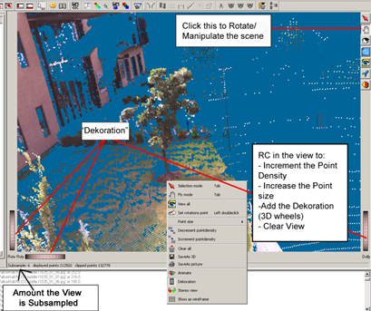
Figure 3: Points to 3D Options

[/wptabcontent]

[wptabtitle]CONTINUE TO…[/wptabtitle]
[wptabcontent]Continue to Z+F Laser Control: Color Mapping[/wptabcontent][/wptabs]

Posted in Laser Control, Scanning, Workflow | Tagged Data Collection, mid-range scanning, Scanning, scanning range >5 meters, Z+F Scanner

Coming Soon!

This document is under development…Please check back soon!

Coming Soon!

This document is under development…Please check back soon!

Coming Soon!

This document is under development…Please check back soon!

Coming Soon!

This document is under development…Please check back soon

Coming Soon!

This document is under development…Please check back soon

Coming Soon!

This document is under development…Please check back soon!

Coming Soon!

This document is under development…Please check back soon

Coming Soon!

This document is under development…Please check back soon

Coming Soon!

This document is under development…Please check back soon

Coming Soon!

This document is under development…Please check back soon

Coming Soon!

This document is under development…Please check back soon

Coming Soon!

This document is under development…Please check back soon!

Coming Soon!

This document is under development…Please check back soon

Who will find this guide useful?

Goal of this Guide

What is the Life Cycle of Your Data?

How are archiving methods related to the end ‘consumption’ of data?

Are accuracy and precision equally important in your data?

How will your data evolve?

Who will find this guide useful?

So, you are now at the point that you are ready to use one or more of these technologies in your project!

Goal of this Guide

How are distance, size of features and data resolution related?

What data resolution do you need?

Which technologies are appropriate for which characteristics?

Additional Qualities to Consider

Physical and Temporal Access to the Site

TIPS

Introducing Polyworks PIFEdit:

Basic Navigation:

Introducing the Optech ILRIS-3D Parser:

Using ILRIS Parser

Add your data

Equipment Checklist – Confirm before leaving the lab!!

1. Tripod – DO NOT FORGET!!!

2. ILRIS 3D Scanner

3. Scanner Batteries – fully charged (4 total)

4. I-Bar/Battery Holder

5. Gray Battery Cable

6. Copy of Operation Manual

7. Operating Options :

8. Optional Equipment:

Why is pre-processing necessary?

Overall steps of this workflow:

Batch RAW to DNG with Adobe Digital Negative (DNG) Converter Software

Steps to Batch Convert:

Batch white balance, image processing, and exporting with Adobe – Part 1: Adobe Bridge

Batch white balance, image processing, and exporting with Adobe – Part 2 : Camera Raw tool

Applying adjustments to all

Saving

General Photography and Close-Range Photogrammetry Standards and Guides