[wptabs mode=”vertical”] [wptabtitle] Why effective resolution?[/wptabtitle] [wptabcontent]For many archaeologists and architects, the minimum size of the features which can be recognized in a 3D model is as important as the reported resolution of the instrument. Normally, the resolution reported for a laser scanner or a photogrammetric project is the point spacing (sometimes referred to as ground spacing distance in aerial photogrammetry). But clearly a point spacing of 5mm does not mean that features 5mm in width will be legible. So it is important that we understand at what resolution features of interest are recognizable, and at what resolution random and instrument noise begin to dominate the model.
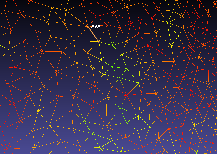
Mesh vertex spacing circa 1cm.
[/wptabcontent]
[wptabtitle] Cloud Compare[/wptabtitle] [wptabcontent]
![]()
![]()
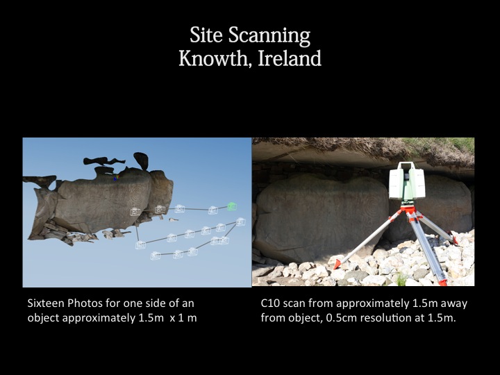
The open source software Cloud Compare, developed by Daniel Girardeau-Montaut, can be used to perform this kind of assessment. The assessment method described here is based on the application of a series of perceptual metrics to 3D models. In this example we compare two 3D models of the same object, one derived from a C10 scanner and one from from a photogrammetric model developed using Agisoft Photoscan.[/wptabcontent]
[wptabtitle] Selecting Test Features[/wptabtitle] [wptabcontent]
Shallow but broad cuttings decorating stones are common features of interest in archaeology. The features here are on the centimetric scale across (in the xy-plane) and on the millimetric scale in depth (z-plane). In this example we assess the resolution at which a characteristic spiral and circles pattern, in this case from the ‘calendar stone’ at Knowth, Ireland is legible, as recorded by a C10 scanner at a nominal 0.5cm point spacing, and by a photogrammetric model built using Agisoft’s photoscan from 16 images.
 [/wptabcontent]
[wptabtitle] Perceptual and Saliency Metrics[/wptabtitle] [wptabcontent]
Models from scanning data of photogrammetry can be both large and complex. Even as models grow in size and complexity, people studying them continue to mentally, subconsciously simplify the model by identifying and extracting the important features.
There are a number of measurements of saliency, or visual attractiveness, of a region of a mesh. These metrics generally incorporate both geometric factors and models of low-level human visual attention.

Local roughness mapped on a subsection of the calendar stone at Knowth.
Roughness is a good example of a relatively simple metric which is an important indicator for mesh saliency. Rough areas are often areas with detail, and areas of concentrated high roughness values are often important areas of the mesh in terms of the recognizability of the essential characteristic features. In the image above you can see roughness values mapped onto the decorative carving, with higher roughness values following the edges of carved areas.
[/wptabcontent]
[wptabtitle] Distribution of Roughness Values[/wptabtitle] [wptabcontent]The presence of roughness isn’t enough. The spatial distribution, or the spatial autocorrelation of the values, is also very important. Randomly distributed small areas with high roughness values usually indicate noise in the mesh. Concentrated, or spatially autocorrelated, areas of high and low roughness in a mesh can indicate a clean model with areas of greater detail.

High roughness values combined with low spatial autocorrelation of these values indicates noise in the model.
[wptabtitle] Picking Relevant Kernel Sizes[/wptabtitle] [wptabcontent]
To use the local roughness values and their distribution to understand the scale at which features are recognizable, we run the metric over our mesh at different, relevant, kernel sizes. In this example, the data in the C10 was recorded at a nominal resolution of 5mm. We run the metric with the kernel at 7mm, 5mm, and 3mm.
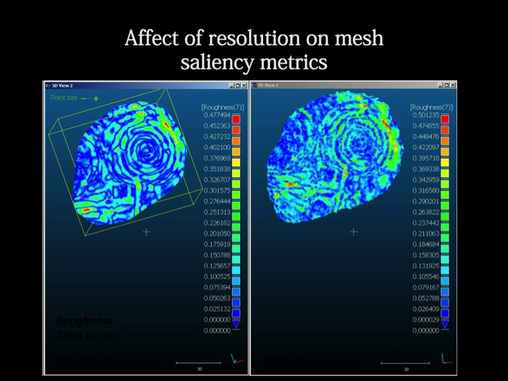
Local roughness value calculated at kernel size: 7mm.
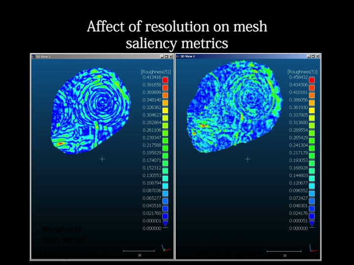
Local roughness value calculated at kernel size: 5mm.
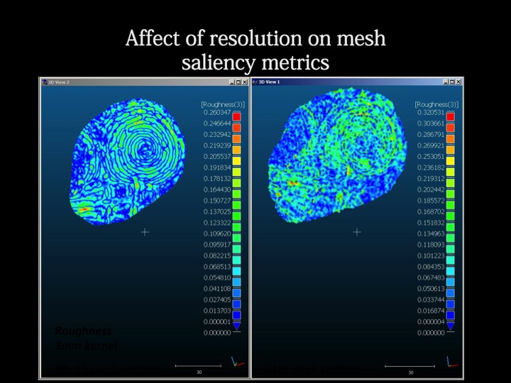
Local roughness value calculated at kernel size: 3mm.
Visually we can see that the distribution of roughness values becomes more random as we move past the effective resolution of the C10 data: 5mm. At 7mm the feature of interest -the characteristic spiral- is clearly visible. At 5mm it is still recognizable, but a little noisy. At 3mm, the picture is dominated by instrument noise.
[/wptabcontent]
[/wptabs]