[wptabs mode=”vertical”] [wptabtitle] Introduction[/wptabtitle] [wptabcontent]
Many archaeological projects use a GIS to manage their data. After terrestrial scan or photogrammetric modeling data has been collected and cleaned, it may be convenient to integrate it into a project’s GIS setup. As ArcGIS is widely available and in use both in University research departments and government offices, we’re using it for the example here, but something like this should work for other GIS packages.
The first part of the workflow addresses working with meshes created from terrestrial scan data, and assumes you have existing meshes in Rapidform.
[/wptabcontent]
[wptabtitle] Decimation[/wptabtitle] [wptabcontent]
Before exporting a dataset for use in a GIS you may want to decimate the dataset to produce a lower resolution model for visualization. High resolution models can slow rendering down and make manipulation of the model difficult.
a. Select the model you will be exporting either graphically or through the menu tree on the left hand side of the screen.
b. In the main menu select Tools and then Scan Tools and Decimate Meshes

Fig. 1: Select the Decimate Meshes tool
c. In the Decimate Meshes menu confirm the selection of the Target Mesh.
d. Under Method choose Poly-Face Count for best control over the size of the resultant model.
e. Under Options set the Target Poly-Face Count. Numbers under 100,000 will render relatively quickly in ArcGIS. Inclusion of more than 500,000 polyfaces is not recommended.
f. Under More Options select Preserve Color.
g. Click “OK” to confirm and decimate the mesh.

Fig. 2: Select options for decimating the mesh.
[/wptabcontent]
[wptabtitle] Subsetting and Splitting Meshes[/wptabtitle] [wptabcontent]
(Skipping ahead a bit conceptually…) When you import your mesh data into ArcGIS each mesh is stored as a single multipatch. You don’t want to edit the shape of the multipatch in ArcGIS, only the placement (trust us on this). So any subsetting of the mesh needs to be performed before exporting from Rapidform (or other modeling software of your choice). Why subset or split a mesh?
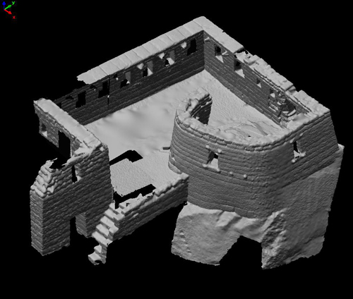
a. Navigating in tight, enclosed spaces. You might want to be able to turn off the visibility of the back wall of a room or one half of a cistern to better visualize its interior.
b. Major sections of a mesh. If you have a scan of a building including several rooms or structures and you want to be able to visualize them individually, then they need to be made into discrete meshes.
[/wptabcontent]
[wptabtitle] Exporting[/wptabtitle] [wptabcontent]
a. Select the model you want to export from the menu tree on the left hand side of the screen.
b. Right-click and select “Export”. Select an appropriate file format (see step 2, below, for choices).

Fig. 3: Export via the menu tree.
4. Export Formats
a. Get a list of valid export formats by looking in the dropdown menu of the export dialog box.

Fig. 4: Valid export file formats.
b. Suggested formats for export are VRML (file extension .wrl), collada (.dae) and AutoDesk 3d Max (.3ds).
[/wptabcontent][wptabtitle] Advice on Textures and Color Data[/wptabtitle] [wptabcontent]
Modeling software manages color data in several ways. Color data might be recorded as UV coordinates referencing a separate texture file, as per vertex, per face or per wedge color information. Color data imported with scan data will typically default to storage as per vertex color. ArcGIS only recognizes color data stored explicitly in texture files, so if your color data is currently stored in another form you need to convert it.
[/wptabcontent]
[wptabtitle] Textures direct from Rapidform[/wptabtitle] [wptabcontent]
i. Select the Mesh mode from the main toolbar.

ii. Select Tools and Texture Tools and Convert Color to Texture. 
Fig. 5: Conver Color to Texture
iii. After creating the texture, export the model as usual.
iv. Export the texture by going in the Main Menu to Texture Tools, then Export Texture to save the texture file. Store it in the same folder as the model.[/wptabcontent]
[wptabtitle] Color and Texture in Meshlab[/wptabtitle] [wptabcontent]Sometimes you want more tools for color editing. Sometimes ArcGIS doesn’t like the textures produced by Rapidform. For this reason, we suggest an alternative method for setting the texture data using Meshlab. Meshlab is open source, and can be found at meshlab.sourceforge.net.
i. From Rapidform export a .VRML file by right-clicking (in the model tree menu on the left land side of the screen) on the mesh you wish to export and selecting Export.
ii. In Meshlab, open a new empty project. Go to File and Import Mesh.

Fig. 6: Import the Mesh to Meshlab
iii. Select the VRML file you just created and hit Open.
iv. Transfer the color information from per vertex to per face. In the main menu go to Filters, then to Color Creation and Processing, then to Transfer Color: Vertex to Face. Hit Apply in the resulting pop-up menu.

Fig. 7: Transfer color data from the vertices to the faces of the mesh.
v. From the Main Menu go to Filters, then to Texture, then to Trivial Per-Triangle Parametrization.

Fig. 8: Create texture data.
In the pop-up menu, select 0 Quads per line, 1024 for the Texture Dimension, and 0 for Inter-Triangle border. Choose the Space Optimizing method. Click Apply.
n.b. If you get an error along the lines of “Inter-Triangle area is too much” your Texture Dimension is too small for the dataset. Increase the texture dimension to resolve the error.

Fig. 9: Set the texture data parameters.
vi. In the Main Menu go to Filters and Texture and Vertex Color to Texture. Accept the defaults for the name and size. Tick the boxes next to Assign texture and Fill Texture.

Fig. 10: Transfer color data to the texture dataset.
vii. In the Main Menu go to File and Export Mesh. Make sure to UNTICK the box next to Vertex Color. Otherwise ArcGIS gets confused! Make sure the texture file is present. Click OK to save.

Fig. 11: Export the mesh as collada (dae).[/wptabcontent]
[wptabtitle] Preparing a GIS to receive Mesh data[/wptabtitle] [wptabcontent]
Once you have created your mesh files and exported them to collada or something similar and explicitly assigned texture data (not to be confused with vertex color, face color or wedge color data), you are ready to import the data into ArcGIS. Assuming your data is not georeferenced, follow the method below. If your data is georeferenced, head over to our Photoscan to ArcGIS post, and follow the import method described there.
1. Preparing the geodatabase
a. Open ArcCatalog any way you choose. Create a new geodatabase by right clicking on the folder where you wish to create the geodatabase and selecting New and File Geodatabase. Only Geodatabases support the import of texture data, so don’t try and use a shapefile.

Fig. 14: Create a geodatabase in ArcGIS.
b. Create a multipatch feature class in the geodatabase.
c. Ensure that the X/Y domain covers the coordinates of any meshes you will be importing. View the Spatial Domain by right-clicking on the feature class and going to Properties and then to the Domain tab.

Fig. 15: Check the spatial domain of the new feature class.
d.If the spatial domain is not suitable, adjust the Environment settings by going to the Geoprocessing toolbar in the Main Menu. Scroll down to Geodatabase Advanced and adjust the Output XY Domain as needed. You can also adjust the Z Domain in this dialog box.

Fig. 16: Adjust the spatial domain in the environment settings.
[/wptabcontent]
[wptabtitle] Preparing the scene file. [/wptabtitle] [wptabcontent]
a. Open ArcScene and add base data such as a plan of the site, an air photo of the location, etc. The base data will allow you to control the location to which the model is imported. Add the empty multipatch feature class you just created.

Fig. 17: Add base data to a Scene.
b. Start editing either from the 3D editor toolbar or by right-clicking on the multipatch feature class in the Table of Contents and choosing Edit Features and Start Editing.

Fig. 18: Start editing in ArcScene. [/wptabcontent][wptabtitle] Importing the Scan data[/wptabtitle] [wptabcontent]
1. Import the vrml or collada file by selecting the Create Features Template for the multipatch and clicking on the base plan roughly in the location where you would like the mesh data to appear. Select the vrml or collada file from the Open File dialog box that appears. Wait while the file is converted.

Fig. 19: The vrml data is converted to multipatch on import.
2. You can now Move, Rotate, Scale the imported multipatch in ArcScene by selecting the feature using the Edit Placement tool and inputting values in the 3D Editing toolbar or by interactively dragging the multipatch feature.

Fig. 20: Select the multipatch feature to adjust its position and scale.
3. Once you are satisfied with the placement of the multipatch, you can add attribute data.
[/wptabcontent]
[wptabtitle] A note on rotation in Arcscene[/wptabtitle] [wptabcontent]
You can only rotate in the x-y plane (that is, around z-axis) in ArcScene. If you need to rotate your data around the x or y axis you need to do this in your modeling software before import. Bringing a .dxf of the polygon or point data you are trying to align the mesh with into your modeling software is probably the simplest way to get the alignment right. You may have to translate your .dxf to a local grid because most modeling software doesn’t like real world coordinates. Losing the real coordinates during this step doesn’t matter because you’re just using the polygon data to set orientation around the x and y axes. You’ll get the model in the correct real-world place when you import into ArcScene.

[/wptabcontent]
[wptabtitle] Re-exporting[/wptabtitle] [wptabcontent]
Fig. 21: The textured mesh data appears over the correct location on the base plan.
4. At this point it’s probably a good idea to re-export a collada model of your newly scaled and located mesh data. If not, every time you update the model you will have to go through the scaling and locating process again.
a. In ArcToolbox go to Conversion Tools> To Collada> Multipatch To Collada. 
Fig. 22: Export Multipatch to Collada
b. Select the multipatch for export and the folder where you want the re-exported model to appear.

Fig. 23: Set parameters for export.
c. Check that the model has exported correctly by opening it in your modeling software.
n.b. You may have to reapply the textures at this point.
[/wptabcontent]
[wptabtitle] A note on features for attribute management [/wptabtitle] [wptabcontent]
It may be convenient to store attribute information in other related feature classes so that a single meshed model can have multiple, spatially discrete attributes. How you design your geodatabase will vary greatly dependent on project requirements.

Fig. 19: Additional related feature classes can be used to manage attribute data.
[/wptabcontent]
[wptabtitle] A note on just how much mesh data you can get into ArcScene.[/wptabtitle] [wptabcontent]
1. If you are using a file geodatabase, in theory the size of the geodatabase is unlimited and you can include all the mesh data you want.
2. In practice, individual meshes with more than 200,000 polygons have problems importing on an average ™ desktop computer.
3. In practice, rendering becomes slow and jumpy with more than 200 MB of mesh data loaded into a single scene on an average ™ desktop computer. The size and quality of your textures will also have an impact here. Compressed textures are probably a good plan.
4. In short, the limitation is on rendering and on what can be cached in an individual scene, rather than on storage in the geodatabase. Consider strategies including having low polygon count meshes for display in a general scene, with links to high polygon count meshes, which can be stored in the geodatabase but not normally rendered in the scene, which can be called up via links in html popup, the attribute table, or via another script.
[/wptabcontent]
[/wptabs]
![clip_image022[6]](https://gmv.cast.uark.edu/wp-content/uploads/2011/06/clip_image0226.jpg "clip_image022[6]") Figure 11 – Piece_001 is fenced and copied to a new MS, using the RP’s as guides; note the fence overlaps slightly beyond the RP, capturing redundant points between adjacent pieces for later re-assembly.
Figure 11 – Piece_001 is fenced and copied to a new MS, using the RP’s as guides; note the fence overlaps slightly beyond the RP, capturing redundant points between adjacent pieces for later re-assembly.![clip_image024[6]](https://gmv.cast.uark.edu/wp-content/uploads/2011/06/clip_image0246.jpg "clip_image024[6]")
![clip_image026[6]](https://gmv.cast.uark.edu/wp-content/uploads/2011/06/clip_image0266.jpg "clip_image026[6]")
![clip_image028[6]](https://gmv.cast.uark.edu/wp-content/uploads/2011/06/clip_image0286.jpg "clip_image028[6]") Figure 14 – Piece_001_A in its own MS, selected and being exported; note the overlap below the RP, creating some redundancy between adjacent scans
Figure 14 – Piece_001_A in its own MS, selected and being exported; note the overlap below the RP, creating some redundancy between adjacent scans![clip_image030[6]](https://gmv.cast.uark.edu/wp-content/uploads/2011/06/clip_image0306.jpg "clip_image030[6]")
![clip_image032[6]](https://gmv.cast.uark.edu/wp-content/uploads/2011/06/clip_image0326.jpg "clip_image032[6]")
![clip_image034[6]](https://gmv.cast.uark.edu/wp-content/uploads/2011/06/clip_image0346.jpg "clip_image034[6]")
![clip_image035[6]](https://gmv.cast.uark.edu/wp-content/uploads/2011/06/clip_image0356.jpg "clip_image035[6]")
![clip_image002[6]](https://gmv.cast.uark.edu/wp-content/uploads/2011/06/clip_image00261.jpg "clip_image002[6]")
![clip_image004[6]](https://gmv.cast.uark.edu/wp-content/uploads/2011/06/clip_image00461.jpg "clip_image004[6]")
![clip_image006[6]](https://gmv.cast.uark.edu/wp-content/uploads/2011/06/clip_image00661.jpg "clip_image006[6]")
![clip_image008[6]](https://gmv.cast.uark.edu/wp-content/uploads/2011/06/clip_image00861.jpg "clip_image008[6]")
![clip_image010[6]](https://gmv.cast.uark.edu/wp-content/uploads/2011/06/clip_image01061.jpg "clip_image010[6]")
![clip_image012[6]](https://gmv.cast.uark.edu/wp-content/uploads/2011/06/clip_image01261.jpg "clip_image012[6]")
![clip_image014[6]](https://gmv.cast.uark.edu/wp-content/uploads/2011/06/clip_image01461.jpg "clip_image014[6]")
![clip_image016[6]](https://gmv.cast.uark.edu/wp-content/uploads/2011/06/clip_image01661.jpg "clip_image016[6]")
![clip_image018[6]](https://gmv.cast.uark.edu/wp-content/uploads/2011/06/clip_image01861.jpg "clip_image018[6]")
![clip_image020[6]](https://gmv.cast.uark.edu/wp-content/uploads/2011/06/clip_image02061.jpg "clip_image020[6]")


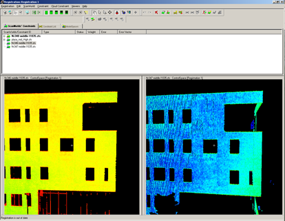 Figure 1: Locking two scan views so that the views rotate/pan/etc… together
 (single pick will erase all other previously picked points in that ScanWorld) and to also ZOOM IN CLOSE when picking points. Also pick points that are spread out across the scan and across different geometries/planar directions. Once the two scan views are aligned to one another, you can also use the Lock button
  to constrain the two views so that they move/rotate together. Once you have selected all of your points, select Constrain from the Cloud Constraints wizard or by going to the Constraint – Add Cloud Constraint. If the Constraint does not work, pick more points and/or remove any bad or incorrect points.NOTE: Cyclone only uses 3 pick points; if you pick 4 or more cyclone will only use the best 3.
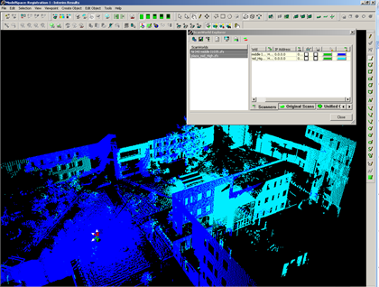 Figure 2: Using the ScanWorld Explorer in a ModelSpace View to assign each scan a unique color
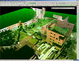 Figure 12: The base XY plane in all Cyclone projects.
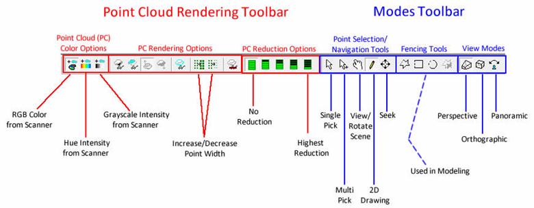
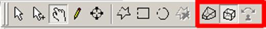 Figure 14: Mode Toolbar shows whether current view is orthogonal or perspective
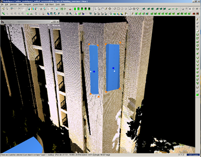 Figure 7: Patches that have been made rectangular

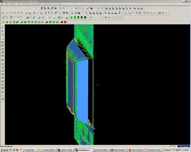 Figure 10: Sub-divided patches can now be deleted, leaving clean corners where patches intersect
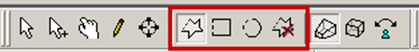 Figure 3: Fence Tools
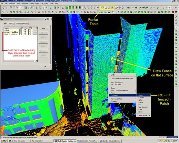 Figure 5: Process of drawing a fence on a flat surface then simply right clicking and selecting Fit Fenced – Patch


![clip_image046[8]](https://gmv.cast.uark.edu/wp-content/uploads/2011/05/clip_image0468.jpg "clip_image046[8]")


![clip_image002[4]](https://gmv.cast.uark.edu/wp-content/uploads/2011/10/clip_image0024.jpg "clip_image002[4]")
![clip_image004[4]](https://gmv.cast.uark.edu/wp-content/uploads/2011/10/clip_image0044.jpg "clip_image004[4]")


![clip_image002[4]](https://gmv.cast.uark.edu/wp-content/uploads/2011/06/clip_image00242.jpg "clip_image002[4]")
![clip_image004[4]](https://gmv.cast.uark.edu/wp-content/uploads/2011/06/clip_image00441.jpg "clip_image004[4]")
![clip_image006[4]](https://gmv.cast.uark.edu/wp-content/uploads/2011/06/clip_image0064.png "clip_image006[4]")
![clip_image008[4]](https://gmv.cast.uark.edu/wp-content/uploads/2011/06/clip_image0084.png "clip_image008[4]")


![clip_image002[6]](https://gmv.cast.uark.edu/wp-content/uploads/2011/06/clip_image0026.jpg "clip_image002[6]")
![clip_image004[6]](https://gmv.cast.uark.edu/wp-content/uploads/2011/06/clip_image0046.jpg "clip_image004[6]")
![clip_image006[6]](https://gmv.cast.uark.edu/wp-content/uploads/2011/06/clip_image0066.jpg "clip_image006[6]")
![clip_image008[6]](https://gmv.cast.uark.edu/wp-content/uploads/2011/06/clip_image0086.jpg "clip_image008[6]")
![clip_image010[6]](https://gmv.cast.uark.edu/wp-content/uploads/2011/06/clip_image0106.jpg "clip_image010[6]")
![clip_image012[6]](https://gmv.cast.uark.edu/wp-content/uploads/2011/06/clip_image0126.jpg "clip_image012[6]")
![clip_image014[6]](https://gmv.cast.uark.edu/wp-content/uploads/2011/06/clip_image0146.jpg "clip_image014[6]")
![clip_image016[6]](https://gmv.cast.uark.edu/wp-content/uploads/2011/06/clip_image0166.jpg "clip_image016[6]")
![clip_image018[6]](https://gmv.cast.uark.edu/wp-content/uploads/2011/06/clip_image0186.jpg "clip_image018[6]")
![clip_image020[6]](https://gmv.cast.uark.edu/wp-content/uploads/2011/06/clip_image0206.jpg "clip_image020[6]")


 ScanWorld: A single scan or collection of scans that are aligned to a common coordinate system. Scanworlds contain ControlSpaces and ModelSpaces.
  ControlSpace : Contains the constraint information used to register multiple scans together.
 ModelSpace: Contains information from the database that has been modeled, process, or changed in some way.
 ModelSpace
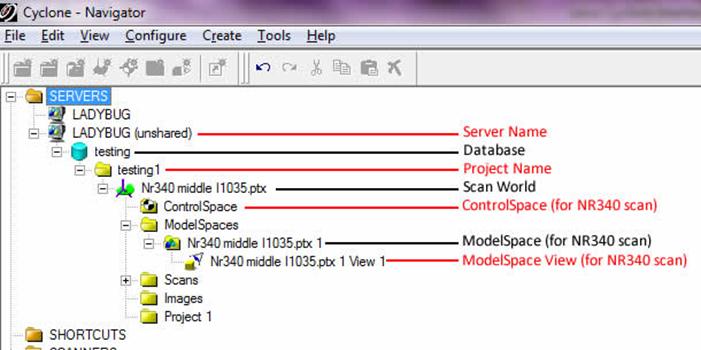