This document will give a brief description of modeling and the modeling tools used in Leica’s Cyclone software..
Hint: You can click on any image to see a larger version.
What is Modeling: The process of creating CAD (Computer-Aided Design) objects. In Cyclone, models are based on 3D point cloud data. CAD models involve more than only shapes as they can also convey information, such as materials, processes, dimensions, and other user-specific details.
To model in Cyclone, you must use:
[wptabs style=”wpui-alma” mode=”vertical”]
[wptabtitle] LAYERS[/wptabtitle]
[wptabcontent]Layers (Shift+L): Layers are used to group similar objects together. This is useful for LOD modeling, controlling object visibility, selectability, etc… ALWAYS model in a layer(s) separate from your original point cloud.
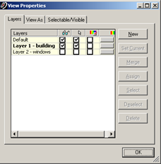
Figure 1: Use the Shift+L button to open the Layers Dialog. Here you can create new layers, set the current layer, and select and assign objects to layers.
[/wptabcontent]
[wptabtitle] FENCES[/wptabtitle]
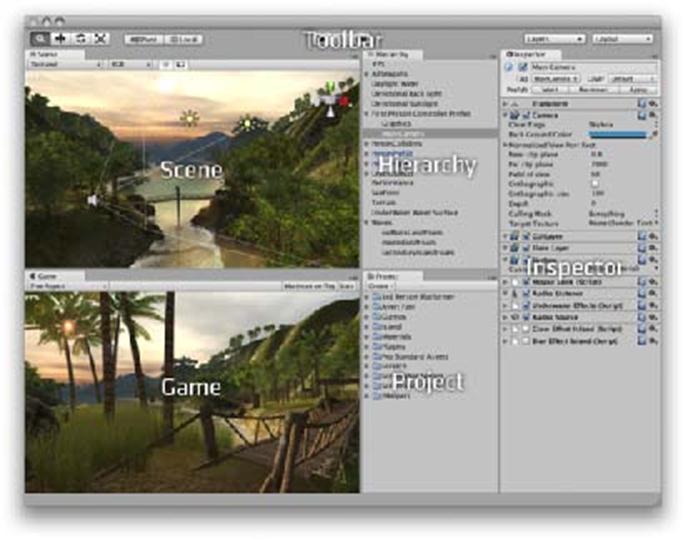
[wptabcontent]Fences: A fence is a 2-dimensional rectangle or polygon that is used as a boundary to select/deselect objects, point clouds, etc…Note: Utilizing the Tool Bar for selection and toggling between modes
will make this much easier rather than navigating through the pull down menus: (Right Click in any part of the menu bar section to pull down the selection list –> Check the Modes selection –> Dock it somewhere on your screen by clicking and dragging). Beware that toolbars “hide” or dock behind others and tend to drift off of the screen. If you can’t locate a toolbar that is listed as showing, drag toolbars to look behind them.
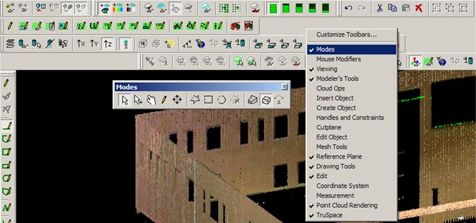 Figure 2: Accessing Toolbars in Cyclone
[/wptabcontent]
[wptabtitle] TEMPORARY MODEL SPACES[/wptabtitle] [wptabcontent]Temporary or “Working” Model Spaces (Select –> RC –> “Copy Fenced to New ModelSpace”): Copying specific areas into temporary or smaller model spaces while modeling allows the user to focus on the pertinent data, making navigation and file handling faster and more efficient. It also allows the user to experiment without threatening the integrity of the original, complete model world. As long as the coordinate system has not been altered, the user can copy/paste (CTRL + C and CTRL + V or Edit –> Copy/Paste) between ModelSpaces and data will transfer in its correct location.
Note: When closing the new “working” model space, the user has the option to “Merge into Original MS” (EVERYthing re-imports, points, objects, etc); “Remove Link from Original MS” (the “working” MS will be saved but will not be associated with the original); or “Delete after close” (the MS and all work in it will be removed). If this dialogue box is closed without a selection, the temporary ModelSpace will be saved in the project with a default name assigned.
Beware: Cyclone does not use a SAVE command; instead, every action is saved, with the option to UNDO, as the user works. It is imortant to pay attention to how model spaces are closed and saved while adjusting to this.
Beware: Cyclone allows multiple ModelSpaces to have the same name leading to confusion if note accounted for.[/wptabcontent]
[wptabtitle] MERGING/UNIFYING POINT CLOUDS[/wptabtitle]
[wptabcontent]Unifying or Merging Multiple Point Clouds: When working with large data sets, it is also recommended to combine the copied point clouds in the working ModelSpace for further ease in navigation and file handling. There are 2 choices for this:
Unify
(Selection –> Select All –> Tools –> Unify Point Clouds): All point clouds are now considered as single cloud in the new “working” model space; note that some functions of the scan world are not maintained with this command.
Merge (Selection –> Select All –> Create Object –> Merge): All point clouds are now considered as single cloud in the new “working” model space; all functions of the scan world are maintained with this command.
[/wptabcontent]
[wptabtitle] CONSTRAINTS[/wptabtitle]
[wptabcontent]Constraints: There are constraints, handles, and snapping functions that aid in the modeling process. Constraints are parameters that the user sets within Cyclone that limit movement, rotation, and drawing tools to specific planes or axes. These parameters regularize and orthagonalize the modeling process. Constraints can be set before the object is created to model more strictly or they can be used with object handles after the obejct is created to manipulate it.
Before Creation: Align the view of the point cloud to the best vantage point of the intended object’s geometry. Viewpoint –> View Lock –> Rotation locks the user’s view to this viewpoint.
Before Creation: Edit Object –> Snapping Grid –> Set Spacing, Rotation, Set to Snap: User can set the spacing of the grid and the rotation to snap to this grid; user can toggle this snap on/off as needed.
During Creation: Tools –> Drawing –> Align Vertices to Axes: toggles on/off the restriction of each vertex to be on the same x or y axes as the previously plotted vertex; after drawing the 1st vertex, the next vertex snaps to the same x or y axis (whichever is closer) as the previous vertex; you may also set the distance to the next vertex here.[/wptabcontent]
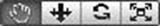
[wptabtitle] HANDLES[/wptabtitle] [wptabcontent]Handles: After creation, objects have a variety of number of handles depending on their geometry. These handles are locations the user can click to grip the object and snap them to manipulate the object’s shape, size, location, and/or rotation. To resize or re-shape
an object –> simply grab and move one of the orange handles located on its perimeter. The blue handle (in the center) is often used to completely translate or move the patch. To add/delete handles –> hold the Alt key when selecting on the handle. Conversely, to add a handle –> hold the Alt key and select along the patch edge.
Handles: Constraints to the Model Space
Edit Object –> Handles –> Show, Constrain Motion, etc…
Edit Object –> Handles –> Edit Snap to Object Threshold: this sets the proximity for snapping handles to objects
Handles: Constraints to Current ActionConstrain handle to specific axis: Select the handle
–> press the x, y, z key
1 time –> handle constrained on this axis
–> press x, y, z key 2nd time –> handle constrained to plane that does not contain that axis
–> press x, y, z key 3rd time –> removes constraint[/wptabcontent]
[wptabtitle] SNAPPING[/wptabtitle] [wptabcontent]Snapping: Snapping allows the user to snap an object’s handle to another object’s handle or to a grid, the spacing of which can be set by the user Edit Object –> Snapping Grid –> Set Spacing.
Snapping Patch Handles: To snap the handles of two adjoining patches together, first select the patch that you are going to SNAP TO then hold the Shift key – grab the handle on the other patch and move it towards the handle that you are snapping to – the two handles should snap together.
[/wptabcontent]
[wptabtitle] OBJECTS, PATCHES & PRIMITIVES[/wptabtitle] [wptabcontent]Objects: There are multiple ways to create objects and meshes. The way that objects are created and the constraints used rely on the user to interpret the scan data and the desired results. This modeling process ranges from precise models that accurately represent the point cloud to highly orthagonal models that less accurately represent the point cloud data but provide more regularized geometries.
Patches: A patch is a plane surface generated from a minimum of 3 points that represents a flat surface that fits to the point cloud. Patches can be extended and grouped to form more complex objects. There are several methods for creating patches.
Primitives (Create Object –> Fit to Cloud or Fit Fenced): Primitive shapes such as cylinders, boxes, and spheres can be fit to point clouds. These objects impose orthagonalized geometry into the modeling process.
Steel Sections/Tables (Create Object –> Fit to Cloud or Fit Fenced): Cyclone allows the user to fit standardized steel sections to the point cloud data to aid in the construction of bridges and any other structures that utilize steel components. After insertion, these sections can be slightly adjusted/customized within a table. Again, these objects/sections impose standardized geometries into the modeling process.
Beware: When an object is created, the object replaces the points that it represents. It is useful to replace or reference these points if more detail or comparisons are needed (this must be done immediately after object is created as the capability is eliminated as modeling progresses)
Select Object –> Right Click –> Insert Copy of Object’s Points or Show Object’s Cloud[/wptabcontent]
[wptabtitle]CONTINUE TO…[/wptabtitle]
[wptabcontent] Continue to Leica Cyclone 7.0: Modeling a Flat Surface … [/wptabcontent]
[/wptabs]
 Check to ensure glass window and lens are free of dust, smudges and fogging. Clean if needed.
 Photograph scanner location if desired.
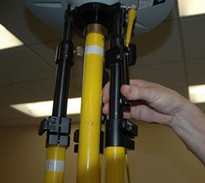
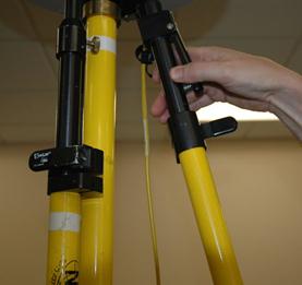
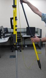
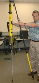
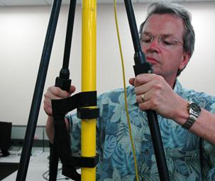
 Set up tripod as level as possible.
 Always pick up scanner with two hands – one ALWAYS on the top handle. Do not let go of the top handle until the scanner is fully secured on the tripod.
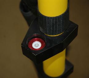
 Level tribrach before turning scanner on.
 Power scanner on.
 Fine tune using digital level in the Level and Laser Plummet menu
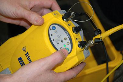
![clip_image003[1]](https://gmv.cast.uark.edu/wp-content/uploads/2011/05/clip_image0031.gif "clip_image003[1]") Create new project: Manage > New. Enter name and press Enter. Click Store button. Click Cont.
Create new project: Manage > New. Enter name and press Enter. Click Store button. Click Cont. Select Scan icon. Click StdStp. DO NOT click ‘Cont’ as this will add more data into STN1.
![clip_image005[1]](https://gmv.cast.uark.edu/wp-content/uploads/2011/05/clip_image0051.gif "clip_image005[1]") Set desired scan field in Fld of View window. Target All = full dome scan.
Set desired scan field in Fld of View window. Target All = full dome scan.![clip_image002[1]](https://gmv.cast.uark.edu/wp-content/uploads/2011/05/clip_image0021.gif "clip_image002[1]") Set desired resolution in Resolution window.
Set desired resolution in Resolution window. Set the image exposure in the ImgCtr window.
![clip_image007[1]](https://gmv.cast.uark.edu/wp-content/uploads/2011/05/clip_image0071.gif "clip_image007[1]") Select Sc+Img or Scan button depending on whether you want to collect color or not.
Select Sc+Img or Scan button depending on whether you want to collect color or not. NEVER take the scanner off the tripod until it has completely shut down and the FAN HAS TURNED OFF*.


 Scanner Positions
 Scan Ranges : full 360
  or defined start and end positions
 No
No  Yes
Yes No
No Yes – Internal
  Yes – External
 17) Scan Forms: Total count
  18) Planimetric map of survey area and scan coverage
 19) Images from survey:
  20) General Notes/Other:


")